
震惊!挖掘了5250篇生命科学领域的文献,我发现了…
本篇推文内容很长,望读者们耐心阅读
今年寒假我没有回家,依然留守科学院工作。繁忙之余,我突然想起来去年11月份刚刚开通微信公众号不久发布的一篇R语言爬虫挖掘illumina接头序列的推文。那篇推文仅仅只是利用R语言爬虫挖掘本地HTML文件数据,在文后我说了后期会发布利用R语言爬虫挖掘网络数据的推文教程。所以,我行思趁现在稍稍有空,我就用R语言爬虫挖掘挖掘一些有用的数据,顺便写这篇推文教大家如何利用R语言爬虫在线数据。
数据挖掘的选择
其实,一开始我只是想挖掘国内生物信息行业招聘数据的。后来我思考了一下2018年中国经济迎来寒冬,互联网科技领域遭受重创,虽然现在新闻说经济又取得多大突破,那确实是有大突破。但是不得不说,我国经济当前下行严重,GDP增速放缓,尤其是遇到2018年中美贸易战,美国对中国互联网科技领域出手,中国的互联网行业受损严重,各大公司裁员,加上2018年大量的印钞票放水,通货膨胀变得相对严重。总之,受各种因素影响,中国在2018年的经济呈现总体发展良好,局部受损严重。但是,各行各业日益紧密联系的今天,互联网行业的受损将以此为中心逐渐向周围行业辐射。这也意味着2019年中国经济也会不乐观。毕竟武汉的地铁价格上涨了50%,全国的药价涨了大约一倍。就算我爬虫挖掘了当下生物信息行业招聘数据,我相信至少在未来三年内,这个行业也不会好挣钱。事实上,我粗略爬虫了一下武汉生物信息行业的平均薪资也就8000多点,其他生物类偏向实验的工作大约6000左右薪资。所以,考虑到开学后也是研一下学期了,准备正式介入自己的课题了,我倒不如爬虫挖掘一些文献期刊数据库。了解了解当前发文章的数据。
PeerJ开源文献期刊数据库爬虫
之所以选择PeerJ开源文献期刊数据库是因为这个数据库涵盖领域广,发文章数量多。关键是,这里面的所有文献都是免费下载!话不多说,直接上图。

我选择了我所学的生命科学领域进行爬虫,在我爬虫的时候PeerJ中共有5250篇生命科学领域的文献,这里面涵盖该领域包括动物学、植物学、微生物学、分子生物学、生物信息学、细胞生物学等多种小领域的文章。每篇链接对应一篇文章,每篇链接内都公开了学术编辑姓名、收稿、审稿、发表时间、作者信息及单位、文章所涉及的相关领域以及文章的关键词,正文等信息。这些都是有用的数据,所以我准备挖掘这些数据,找出PeerJ期刊中都有哪些学术编辑?他们中哪些人审稿生物信息学相关的文章?每个人通常会审稿文章多少时间?另外还想挖掘一下生物信息学目前都在哪些领域用到?也就是和生物信息学有直接交集的领域都有哪些?还有从2016年到现在生物信息学领域都有哪些研究热点?最后还想挖掘文章作者及单位的国家数据。
要挖掘这些数据,首先要找到这些数据在HTML中对应CSS路径,具体方法可以见我上一篇R语言爬虫中的教程(点击阅读原文可见)。还是使用Google的SelectorGadget插件进行路径查找

爬虫同样使用R语言的rvest函数包,将爬取的数据以文本形式传递,再用正则表达式进行过滤,保留有效数据。毕竟正则表达式是人类语言的抽象哲学。首先爬虫文章的领域、编辑、作者单位和审稿时间、文章关键词等信息
#爬虫挖掘相关数据并过滤整理
library(rvest)
PeerJField<-NULL
PeerJEditor<-NULL
PeerJPaper<-NULL
Author_country<-NULL
Paper_time<-NULL
Paper_keyword<-list()
for (i in 1:350) {
  url<-paste("https://peerj.com/articles/?journal=peerj&discipline=biology&q=&page=",i,sep = "")
  myPeerj<-read_html(url)
  peerjfield<-myPeerj%>%
    html_nodes(css = ".main-search-item-subjects")%>%
    html_text()
  peerjeditor<-myPeerj%>%
    html_nodes(css = ".main-search-item-editor .search-item-show-link")%>%
    html_text()
  peerjpaper<-myPeerj%>%
    html_nodes(css = "#wrap .span5")%>%
    html_text()
  peerjeditor<-gsub(pattern = "E\n",replacement = "",peerjeditor)
  peerjeditor<-gsub(pattern = "\n",replacement = "",peerjeditor)
  peerjeditor<-gsub(pattern = " ",replacement = "",peerjeditor)
  peerjfield<-gsub(pattern = "\\[",replacement = "",peerjfield)
  peerjfield<-gsub(pattern = "\\]",replacement = "",peerjfield)
  peerjfield<-gsub(pattern = "\"",replacement = "",peerjfield,fixed = TRUE)
  peerjpaper<-gsub(pattern = "\n",replacement = "",peerjpaper)
  peerjpaper<-gsub(pattern = " ",replacement = "",peerjpaper)
  peerjpaper<-gsub(pattern = ":[0-9]+.[0-9]+",replacement = "",peerjpaper)
  peerjpaper<-gsub(pattern = "[A-Za-z]+/peerj.",replacement = "",peerjpaper)
  peerjpaper<-gsub(pattern = "[A-Za-z]+-",replacement = "",peerjpaper)
  peerjpaper<-gsub(pattern = "[A-Za-z]+.",replacement = "",peerjpaper)
  peerjpaper<-gsub(pattern = "[\u00C0-\u00FF]+",replacement = "",peerjpaper)
  PeerJField<-c(PeerJField,peerjfield)
  PeerJEditor<-c(PeerJEditor,peerjeditor)
  PeerJPaper<-c(PeerJPaper,peerjpaper)
}
for (j in 1:length(PeerJPaper)) {
  url2<-paste("https://peerj.com/articles/",PeerJPaper[j],sep = "")
  myPeerj<-read_html(url2)
  author<-myPeerj%>%
    html_nodes(css = ".country")%>%
    html_text()
  time<-myPeerj%>%
    html_nodes(css = "#article-information time")%>%
    html_text()
  keywords<-myPeerj%>%
    html_nodes(css = ".kwd")%>%
    html_text()
  keywords<-gsub(pattern = "  ",replacement = "",keywords)
  keywords<-gsub(pattern = "\n",replacement = "",keywords)
  Paper_keyword[[j]]<-keywords
  Author_country<-c(Author_country,author)
  Paper_time<-rbind(Paper_time,time)
}
TotalPaperdata<-data.frame(Field=PeerJField,editor=PeerJEditor,Accepted=Paper_time[,2],Received=Paper_time[,3])
PeerJField_list<-strsplit(PeerJField,",")
生物信息学类文章编辑审稿时间分析
我认为,就算是同样的期刊,不同的学术编辑可能对文章的把控严度不同。虽然一篇文章会由多个人审核,但是学术编辑只有一个,他对文章的把持也是非常重要的,我琢磨能不能通过分析这些学术编辑审稿时间来判断投稿时遇到不同编辑文章的过审时间可能有多长,于是我通过分析多篇生物信息学文章的学术编辑姓名还有文章的审稿时间(这个时间我通过Received time和Accepted time之差来判断),我将所有审稿数量大于等于3篇的学术编辑进行了审稿时间分析
#生物信息学类文章编辑审稿时间分析
BIEditor_list<-list()
i<-1
while (i<=nrow(TotalPaperdata)) {
  field_editor<-strsplit(as.character(TotalPaperdata[i,1]),",")[[1]]
  if(length(intersect(c("Bioinformatics","Data Science"),field_editor))>=1){
    BIEditor_list[[as.character(TotalPaperdata[i,2])]]<-c(BIEditor_list[[as.character(TotalPaperdata[i,2])]],
                                                          as.numeric(as.Date(TotalPaperdata[i,3])-as.Date(TotalPaperdata[i,4])))}
  i=i+1
}
plotBIEditor_list<-list()
i<-1
while (i<=length(BIEditor_list)) {
  if(length(BIEditor_list[[i]])>=3){
    plotBIEditor_list<-c(plotBIEditor_list,BIEditor_list[i])
  }
  i=i+1
}
BIEditor_name<-NULL
BIEditor_time<-NULL
BIEditor_checkpaper<-data.frame()
for (i in 1:length(plotBIEditor_list)) {
  BIEditor_name<-names(plotBIEditor_list[i])
  for(j in 1:length(plotBIEditor_list[[i]])){
    BIEditor_time<-data.frame(name=BIEditor_name,time=plotBIEditor_list[[i]][j])
    BIEditor_checkpaper<-rbind(BIEditor_checkpaper,BIEditor_time)
  }
}
library(ggplot2)
p<-ggplot(data = BIEditor_checkpaper,mapping = aes(x=BIEditor_checkpaper$name,y=BIEditor_checkpaper$time,fill=factor(BIEditor_checkpaper$name)),)+
  geom_boxplot()+
  theme(axis.text.x = element_text(angle = 75, hjust = 0.5, vjust = 0.5,size = 8))+
  guides(fill=FALSE)+
  labs(title="Edit review time in BI&DM article",x=NULL,y=NULL)+
  theme(text = element_text(color = "Black"),
        plot.title = element_text(size=15,color = "Black"),
        panel.background = element_blank(),
        panel.border = element_blank(),
        panel.grid.major = element_blank(),
        panel.grid.minor = element_blank())

从结果中看出,大多数审稿生物信息学文章的学术编辑审稿平均时间在100天左右,也有不少审稿时间小于60天,个别还有40多天的审稿时间,但是2~3个学术编辑的审稿时间非常长,平均在300天(也就是一年),有一篇文章居然花了600多天才审核过。当然,单纯以学术编辑和审稿时间来判断学术编辑是否审稿时间长并不严谨,这部分数据只能反映多数编辑的审稿时间在3个月左右。审稿时间也可能受补充实验时长影响,毕竟有的文章不只有生物信息学分析还有很多实验。补实验确实是一个非常费时间的过程。不过在文章质量保证的情况下,我们遇到这里面审稿平均时间短的学术编辑审稿可能会较快过审。
研究方向关联网络分析
毕竟发纯生物信息学文章的数量不多,很多文章都是结合生物信息学和实验一起发的,而通过挖掘这部分数据也可以大致了解当前有哪些领域较多地应用生物信息学
#研究方向关联网络分析
Networkfield<-NULL
i<-1
while (i<=length(PeerJField_list)) {
  netfield<-NULL
  for (j in 1:(length(PeerJField_list[[i]])-1)) {
    for (k in (j+1):length(PeerJField_list[[i]])) {
      field<-c(as.character(PeerJField_list[[i]][j]),as.character(PeerJField_list[[i]][k]))
      netfield<-rbind(netfield,field)
    }
  }
  Networkfield<-rbind(Networkfield,netfield)
  i=i+1
}
Networkfield<-data.frame(Networkfield)
library(networkD3)
library(DMwR)
networkfield<-na.omit(Networkfield)
simpleNetwork(networkfield[1:2100,],fontSize = 14,nodeColour = "red",
              linkDistance=300,zoom = T)
simpleNetwork(networkfield)
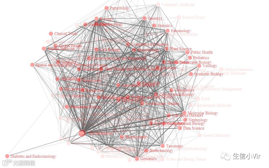
由于数据较多,我只画了2100个列子,通过网络图的可视化结果看出,当前生物信息学主要在基因组学、免疫学、全球健康、遗传学、分类学、统计学、数据挖掘、机器学习、公共健康、细胞生物学、植物科学、合成生物学等大量的领域有应用,可以看出当前生物信息学具有非常广泛的用途。拥有生物信息学扎实功底的人能在更广的领域有作用!
生物信息学领域文章关键词分析
当然,仅仅有这些数据还不够,还需要关注近几年生物信息学领域都在关注什么问题,这样才有助于我们抓住生物信息学的热点。所以我把从2016年到今天的所有PeerJ上发表的生物信息学相关的文章的关键词取词频超过3次的词汇进行词云可视化
#生物信息学领域文章关键词分析
BIkeyword_list<-list()
i<-1
NewTotalPaperdata<-data.frame()
while (i<=nrow(TotalPaperdata)) {
  if(as.numeric(as.Date(TotalPaperdata[i,4])-as.Date("2016-01-01"))>=0){
    NewTotalPaperdata<-rbind(NewTotalPaperdata,TotalPaperdata[i,])
  }
  i=i+1
}
i<-1
while (i<=length(Paper_keyword)) {
  field_editor<-strsplit(as.character(NewTotalPaperdata[i,1]),",")[[1]]
  if(length(intersect(c("Bioinformatics","Data Science"),field_editor))>=1){
    BIkeyword_list<-c(BIkeyword_list,Paper_keyword[i])}
  else{BIkeyword_list<-BIkeyword_list}
  i=i+1
}
BIkeywd_list<-list()
BIkeyword_table<-NULL
for (i in 1:length(BIkeyword_list)) {
  keyword<-BIkeyword_list[[i]]
  for (j in 1:length(keyword)) {
    keywd<-strsplit(keyword[j]," ")[[1]]
    for (k in 1:length(keywd)) {
      BIkeywd_list[[keywd[k]]]<-c(BIkeywd_list[[keywd[k]]],1)
    }
  }
}
BIkeywd<-names(BIkeywd_list)
BIkeywdN<-NULL
for (i in 1:length(BIkeywd)) {
  BIkeywdN<-c(BIkeywdN,sum(BIkeywd_list[[BIkeywd[i]]]))
}
BIkeyword_table<-data.frame(keyword=BIkeywd,number=BIkeywdN)
plotBIkeyword_table<-BIkeyword_table[BIkeyword_table$number>3,]
library(wordcloud2)
wordcloud2(plotBIkeyword_table,size = 1,shape = 'dimond')
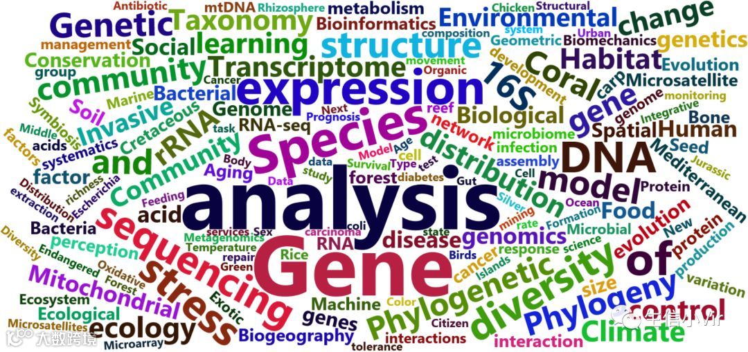
从结果中看出,从2016年到现在,分析方法、测序技术、转录组、基因组、16srRNA、分类学、肠道微生物、微生物组学、宏基因组学、机器学习以及生态学都是很热点的内容。不过根据我的经验,2016年和2017年是转录组文章产量非常高的年份,所以还需要进一步分析每年甚至是每个月的热点,才能有效把握最新热点。
研究领域发文量分析
除了关注生物信息学的发文情况,再把目光转移到各个生物学领域上,将PeerJ内的所有文章按照研究领域分类,进行发文数量的分析
#研究领域发文量分析
TotalField<-data.frame()
totalfield_list<-list()
i<-1
while (i<=nrow(TotalPaperdata)) {
  field<-strsplit(as.character(TotalPaperdata[i,1]),",")[[1]]
  for (j in 1:length(field)) {
    fd<-field[j]
    totalfield_list[[fd]]<-c(totalfield_list[[fd]],1)
  }
  i=i+1
}
field_name<-names(totalfield_list)
field_number<-NULL
for (i in 1:length(totalfield_list)) {
  field_number<-c(field_number,sum(totalfield_list[[i]]))
}
TotalField<-data.frame(field=field_name,number=field_number)
plotField<-TotalField[TotalField$number>4,]
library(ggplot2)
pic<-ggplot(data = plotField,mapping = aes(x=field,y=number,fill=field),)+
  geom_bar(stat = "identity",width = 1)+
  guides(fill=FALSE)+coord_flip()+
  labs(x=NULL,y=NULL)+
  theme(text = element_text(color = "Black"),
        axis.text.x=element_text(face="bold",size=10,angle=0,color="Black"),
        axis.text.y=element_text(face="bold",size=5,angle=0,color="Black"),
        plot.title = element_text(size=10,color = "Black"),
        panel.background = element_blank(),
        panel.border = element_blank(),
        panel.grid.major = element_blank(),
        panel.grid.minor = element_blank())

从结果中看出,最高的发文量还是以动物学这些一级学科,不过这里面涵盖了很多二级学科,以二级学科分类生物信息学的发文量是非常高的,基因组学、细胞生物学、生态学等发文量也非常高。从之前的关联网络分析结果可以推测这些学科的发文量也有生物信息学的推动。
作者单位国籍分析
文章都有作者所在单位的信息,继续挖掘一下作者单位信息,先看看这些单位都是来自哪些国家的,通过这些信息也可以反映国家科研实力的表面强弱
#作者单位国籍分析
author_country<-Author_country
for(j in 1:length(author_country)){
  if(grepl(pattern = "China",author_country[j])){
    author_country[j]<-"China"
  }
  else if(grepl(pattern = "Taiwan",author_country[j])){
    author_country[j]<-"China"
  }
  else if(grepl(pattern = "America",author_country[j])){
    author_country[j]<-"USA"
  }
  else if(grepl(pattern = "United States",author_country[j])){
    author_country[j]<-"USA"
  }
  else if(grepl(pattern = "United Kingdom",author_country[j])){
    author_country[j]<-"UK"
  }
  else if(grepl(pattern = "Uk",author_country[j])){
    author_country[j]<-"UK"
  }
}
author_country<-gsub(pattern = " ",replacement = "",author_country)
authorcontry_list<-list()
i<-1
while (i<=length(author_country)) {
  country<-author_country[i]
  authorcontry_list[[country]]<-c(authorcontry_list[[country]],1)
  i=i+1
}
Nation<-names(authorcontry_list)
AUTHor<-NULL
for (j in 1:length(authorcontry_list)) {
  AUTHor<-c(AUTHor,sum(authorcontry_list[[j]]))
}
Author_data<-data.frame(national=Nation,author_number=AUTHor)
plotAuthor_data<-Author_data[Author_data$author_number>30,]
library(ggplot2)
pic<-ggplot(data = plotAuthor_data,mapping = aes(x=national,y=author_number,fill=national),)+
  geom_bar(stat = "identity",width = 0.9,)+
  guides(fill=FALSE)+coord_flip()+
  labs(x=NULL,y=NULL)+
  theme(text = element_text(color = "Black"),
        axis.text.x=element_text(face="bold",size=10,angle=0,color="Black"),
        axis.text.y=element_text(face="bold",size=8,angle=0,color="Black"),
        plot.title = element_text(size=10,color = "Black"),
        panel.background = element_blank(),
        panel.border = element_blank(),
        panel.grid.major = element_blank(),
        panel.grid.minor = element_blank())

从分析结果看,美国的科研单位参与数量最多有4000多家,一方面可能因为美国发文多,还有一方面也是因为科研单位之间的合作密切,数据公开共享程度高。中国的科研单位参与量是美国的一半,一方面可能是因为中国是近几年才在科技领域有很大突破,也有一部分原因还是因为国内科研单位合作不密切,共享度低。
平均每篇文章的作者数量
一篇文章会有很多个作者。当然,明白人都知道,一篇文章除了一二作者和通讯作者外,其他作者几乎都是挂名没啥实际贡献。除非是一些高水平文章。分析文章作者的数量可以分析一下科研圈的裙带关系
#平均每篇文章的作者数量
PeerJAuCu<-data.frame()
for(i in 1:length(PeerJPaper)){
  url3<-paste("https://peerj.com/articles/",PeerJPaper[i],sep = "")
  mypj<-read_html(url3)
  peerjaucu<-mypj%>%
    html_nodes(css = ".article-authors , .country")%>%
    html_text()
  peerjaucu<-peerjaucu[1:2]
  peerjcu<-peerjaucu[2]
  if(grepl(pattern = "China",peerjcu)){
    peerjcu<-"China"
  }else if(grepl(pattern = "P. R. China",peerjcu)){
    peerjcu<-"China"}else if(grepl(pattern = "America",peerjcu)){
        peerjcu<-"USA"}else if(grepl(pattern = "United States",peerjcu)){peerjcu<-"USA"}else if(grepl(pattern = "United Kingdom",peerjcu)){
          peerjcu<-"UK"}else if(grepl(pattern = "Uk",peerjcu)){
            peerjcu<-"UK"}
  peerjau<-strsplit(peerjaucu[1],", ")[[1]]
  peerjau<-gsub(pattern = "[0-9]+",replacement = "",peerjau)
  peerjau<-gsub(pattern = ",",replacement = "",peerjau)
  peerjau<-gsub(pattern = "\n",replacement = "",peerjau)
  peerjaunumber<-length(peerjau)
  peerj_aucu<-data.frame(Author_number=peerjaunumber,national=peerjcu)
  PeerJAuCu<-rbind(PeerJAuCu,peerj_aucu)
}
PeerJ_AuCu<-PeerJAuCu[PeerJAuCu$national %in%
                        c("China","Japan","USA","Australia","Russia","UK","Germany","Finland","India",
                          "Italy","Canada","Hungary","France"),]
library(ggplot2)
p<-ggplot(data = PeerJ_AuCu,mapping = aes(x=national,y=Author_number,))+
  geom_boxplot(aes(fill=factor(national)),width=0.5)+guides(fill=FALSE)+
  theme(text = element_text(color = "Black"),
        axis.text.x=element_text(size=10,angle=0,color="Black"),
        axis.text.y=element_text(size=10,angle=0,color="Black"),
        plot.title = element_text(size=10,color = "Black"))

有趣的是,这个结果直接显示出了中国平均每篇文章的作者数量最多,基本上等于其他国家的上25%分位数,大约有7个,可以说肯定是有部分的裙带关系迹象的,毕竟也是理解,实验室老师之间的文章互带可以给他们带来一些利益。但是我认为,考虑到中国的科研单位参与文章发文量相对也不少,这也是中国平均每篇文章作者数量多的一个原因。但是看看美国,我感觉也不咋样,美国的文章虽然平均一篇文章作者数量较少,但是也存在很多极端值。不过总体来看,白人国家的优等白人和日本人平均一篇文章带作者少。不过这个结论必须要考虑文章质量,篇均被引次数等再下定论,现在的结论只是粗糙模糊结论。
代码总结
这次分析总共只有272行代码,现总结在这里便于学习。希望自己以后还能挖掘出更多的文献数据信息。我认为挖掘文献数据是一个非常有用的内容,这能够为实验室发文章,抓研究热点提供非常可靠的信息。
library(rvest)
PeerJField<-NULL
PeerJEditor<-NULL
PeerJPaper<-NULL
Author_country<-NULL
Paper_time<-NULL
Paper_keyword<-list()
for (i in 1:350) {
  url<-paste("https://peerj.com/articles/?journal=peerj&discipline=biology&q=&page=",i,sep = "")
  myPeerj<-read_html(url)
  peerjfield<-myPeerj%>%
    html_nodes(css = ".main-search-item-subjects")%>%
    html_text()
  peerjeditor<-myPeerj%>%
    html_nodes(css = ".main-search-item-editor .search-item-show-link")%>%
    html_text()
  peerjpaper<-myPeerj%>%
    html_nodes(css = "#wrap .span5")%>%
    html_text()
  peerjeditor<-gsub(pattern = "E\n",replacement = "",peerjeditor)
  peerjeditor<-gsub(pattern = "\n",replacement = "",peerjeditor)
  peerjeditor<-gsub(pattern = " ",replacement = "",peerjeditor)
  peerjfield<-gsub(pattern = "\\[",replacement = "",peerjfield)
  peerjfield<-gsub(pattern = "\\]",replacement = "",peerjfield)
  peerjfield<-gsub(pattern = "\"",replacement = "",peerjfield,fixed = TRUE)
  peerjpaper<-gsub(pattern = "\n",replacement = "",peerjpaper)
  peerjpaper<-gsub(pattern = " ",replacement = "",peerjpaper)
  peerjpaper<-gsub(pattern = ":[0-9]+.[0-9]+",replacement = "",peerjpaper)
  peerjpaper<-gsub(pattern = "[A-Za-z]+/peerj.",replacement = "",peerjpaper)
  peerjpaper<-gsub(pattern = "[A-Za-z]+-",replacement = "",peerjpaper)
  peerjpaper<-gsub(pattern = "[A-Za-z]+.",replacement = "",peerjpaper)
  peerjpaper<-gsub(pattern = "[\u00C0-\u00FF]+",replacement = "",peerjpaper)
  PeerJField<-c(PeerJField,peerjfield)
  PeerJEditor<-c(PeerJEditor,peerjeditor)
  PeerJPaper<-c(PeerJPaper,peerjpaper)
}
for (j in 1:length(PeerJPaper)) {
  url2<-paste("https://peerj.com/articles/",PeerJPaper[j],sep = "")
  myPeerj<-read_html(url2)
  author<-myPeerj%>%
    html_nodes(css = ".country")%>%
    html_text()
  time<-myPeerj%>%
    html_nodes(css = "#article-information time")%>%
    html_text()
  keywords<-myPeerj%>%
    html_nodes(css = ".kwd")%>%
    html_text()
  keywords<-gsub(pattern = "  ",replacement = "",keywords)
  keywords<-gsub(pattern = "\n",replacement = "",keywords)
  Paper_keyword[[j]]<-keywords
  Author_country<-c(Author_country,author)
  Paper_time<-rbind(Paper_time,time)
}
TotalPaperdata<-data.frame(Field=PeerJField,editor=PeerJEditor,Accepted=Paper_time[,2],Received=Paper_time[,3])
PeerJField_list<-strsplit(PeerJField,",")
#生物信息学类文章编辑审稿时间分析
BIEditor_list<-list()
i<-1
while (i<=nrow(TotalPaperdata)) {
  field_editor<-strsplit(as.character(TotalPaperdata[i,1]),",")[[1]]
  if(length(intersect(c("Bioinformatics","Data Science"),field_editor))>=1){
    BIEditor_list[[as.character(TotalPaperdata[i,2])]]<-c(BIEditor_list[[as.character(TotalPaperdata[i,2])]],
                                                          as.numeric(as.Date(TotalPaperdata[i,3])-as.Date(TotalPaperdata[i,4])))}
  i=i+1
}
plotBIEditor_list<-list()
i<-1
while (i<=length(BIEditor_list)) {
  if(length(BIEditor_list[[i]])>=3){
    plotBIEditor_list<-c(plotBIEditor_list,BIEditor_list[i])
  }
  i=i+1
}
BIEditor_name<-NULL
BIEditor_time<-NULL
BIEditor_checkpaper<-data.frame()
for (i in 1:length(plotBIEditor_list)) {
  BIEditor_name<-names(plotBIEditor_list[i])
  for(j in 1:length(plotBIEditor_list[[i]])){
    BIEditor_time<-data.frame(name=BIEditor_name,time=plotBIEditor_list[[i]][j])
    BIEditor_checkpaper<-rbind(BIEditor_checkpaper,BIEditor_time)
  }
}
library(ggplot2)
p<-ggplot(data = BIEditor_checkpaper,mapping = aes(x=BIEditor_checkpaper$name,y=BIEditor_checkpaper$time,fill=factor(BIEditor_checkpaper$name)),)+
  geom_boxplot()+
  theme(axis.text.x = element_text(angle = 75, hjust = 0.5, vjust = 0.5,size = 8))+
  guides(fill=FALSE)+
  labs(title="Edit review time in BI&DM article",x=NULL,y=NULL)+
  theme(text = element_text(color = "Black"),
        plot.title = element_text(size=15,color = "Black"),
        panel.background = element_blank(),
        panel.border = element_blank(),
        panel.grid.major = element_blank(),
        panel.grid.minor = element_blank())
#研究方向关联网络分析
Networkfield<-NULL
i<-1
while (i<=length(PeerJField_list)) {
  netfield<-NULL
  for (j in 1:(length(PeerJField_list[[i]])-1)) {
    for (k in (j+1):length(PeerJField_list[[i]])) {
      field<-c(as.character(PeerJField_list[[i]][j]),as.character(PeerJField_list[[i]][k]))
      netfield<-rbind(netfield,field)
    }
  }
  Networkfield<-rbind(Networkfield,netfield)
  i=i+1
}
Networkfield<-data.frame(Networkfield)
library(networkD3)
library(DMwR)
networkfield<-na.omit(Networkfield)
simpleNetwork(networkfield[1:2100,],fontSize = 14,nodeColour = "red",
              linkDistance=300,zoom = T)
simpleNetwork(networkfield)
#生物信息学领域文章关键词分析
BIkeyword_list<-list()
i<-1
NewTotalPaperdata<-data.frame()
while (i<=nrow(TotalPaperdata)) {
  if(as.numeric(as.Date(TotalPaperdata[i,4])-as.Date("2016-01-01"))>=0){
    NewTotalPaperdata<-rbind(NewTotalPaperdata,TotalPaperdata[i,])
  }
  i=i+1
}
i<-1
while (i<=length(Paper_keyword)) {
  field_editor<-strsplit(as.character(NewTotalPaperdata[i,1]),",")[[1]]
  if(length(intersect(c("Bioinformatics","Data Science"),field_editor))>=1){
    BIkeyword_list<-c(BIkeyword_list,Paper_keyword[i])}
  else{BIkeyword_list<-BIkeyword_list}
  i=i+1
}
BIkeywd_list<-list()
BIkeyword_table<-NULL
for (i in 1:length(BIkeyword_list)) {
  keyword<-BIkeyword_list[[i]]
  for (j in 1:length(keyword)) {
    keywd<-strsplit(keyword[j]," ")[[1]]
    for (k in 1:length(keywd)) {
      BIkeywd_list[[keywd[k]]]<-c(BIkeywd_list[[keywd[k]]],1)
    }
  }
}
BIkeywd<-names(BIkeywd_list)
BIkeywdN<-NULL
for (i in 1:length(BIkeywd)) {
  BIkeywdN<-c(BIkeywdN,sum(BIkeywd_list[[BIkeywd[i]]]))
}
BIkeyword_table<-data.frame(keyword=BIkeywd,number=BIkeywdN)
plotBIkeyword_table<-BIkeyword_table[BIkeyword_table$number>3,]
library(wordcloud2)
wordcloud2(plotBIkeyword_table,size = 1,shape = 'dimond')
#研究领域发文量分析
TotalField<-data.frame()
totalfield_list<-list()
i<-1
while (i<=nrow(TotalPaperdata)) {
  field<-strsplit(as.character(TotalPaperdata[i,1]),",")[[1]]
  for (j in 1:length(field)) {
    fd<-field[j]
    totalfield_list[[fd]]<-c(totalfield_list[[fd]],1)
  }
  i=i+1
}
field_name<-names(totalfield_list)
field_number<-NULL
for (i in 1:length(totalfield_list)) {
  field_number<-c(field_number,sum(totalfield_list[[i]]))
}
TotalField<-data.frame(field=field_name,number=field_number)
plotField<-TotalField[TotalField$number>4,]
library(ggplot2)
pic<-ggplot(data = plotField,mapping = aes(x=field,y=number,fill=field),)+
  geom_bar(stat = "identity",width = 1)+
  guides(fill=FALSE)+coord_flip()+
  labs(x=NULL,y=NULL)+
  theme(text = element_text(color = "Black"),
        axis.text.x=element_text(face="bold",size=10,angle=0,color="Black"),
        axis.text.y=element_text(face="bold",size=5,angle=0,color="Black"),
        plot.title = element_text(size=10,color = "Black"),
        panel.background = element_blank(),
        panel.border = element_blank(),
        panel.grid.major = element_blank(),
        panel.grid.minor = element_blank())
#作者单位国籍分析
author_country<-Author_country
for(j in 1:length(author_country)){
  if(grepl(pattern = "China",author_country[j])){
    author_country[j]<-"China"
  }
  else if(grepl(pattern = "Taiwan",author_country[j])){
    author_country[j]<-"China"
  }
  else if(grepl(pattern = "America",author_country[j])){
    author_country[j]<-"USA"
  }
  else if(grepl(pattern = "United States",author_country[j])){
    author_country[j]<-"USA"
  }
  else if(grepl(pattern = "United Kingdom",author_country[j])){
    author_country[j]<-"UK"
  }
  else if(grepl(pattern = "Uk",author_country[j])){
    author_country[j]<-"UK"
  }
}
author_country<-gsub(pattern = " ",replacement = "",author_country)
authorcontry_list<-list()
i<-1
while (i<=length(author_country)) {
  country<-author_country[i]
  authorcontry_list[[country]]<-c(authorcontry_list[[country]],1)
  i=i+1
}
Nation<-names(authorcontry_list)
AUTHor<-NULL
for (j in 1:length(authorcontry_list)) {
  AUTHor<-c(AUTHor,sum(authorcontry_list[[j]]))
}
Author_data<-data.frame(national=Nation,author_number=AUTHor)
plotAuthor_data<-Author_data[Author_data$author_number>30,]
library(ggplot2)
pic<-ggplot(data = plotAuthor_data,mapping = aes(x=national,y=author_number,fill=national),)+
  geom_bar(stat = "identity",width = 0.9,)+
  guides(fill=FALSE)+coord_flip()+
  labs(x=NULL,y=NULL)+
  theme(text = element_text(color = "Black"),
        axis.text.x=element_text(face="bold",size=10,angle=0,color="Black"),
        axis.text.y=element_text(face="bold",size=8,angle=0,color="Black"),
        plot.title = element_text(size=10,color = "Black"),
        panel.background = element_blank(),
        panel.border = element_blank(),
        panel.grid.major = element_blank(),
        panel.grid.minor = element_blank())
#平均每篇文章的作者数量
PeerJAuCu<-data.frame()
for(i in 1:length(PeerJPaper)){
  url3<-paste("https://peerj.com/articles/",PeerJPaper[i],sep = "")
  mypj<-read_html(url3)
  peerjaucu<-mypj%>%
    html_nodes(css = ".article-authors , .country")%>%
    html_text()
  peerjaucu<-peerjaucu[1:2]
  peerjcu<-peerjaucu[2]
  if(grepl(pattern = "China",peerjcu)){
    peerjcu<-"China"
  }else if(grepl(pattern = "P. R. China",peerjcu)){
    peerjcu<-"China"}else if(grepl(pattern = "America",peerjcu)){
        peerjcu<-"USA"}else if(grepl(pattern = "United States",peerjcu)){peerjcu<-"USA"}else if(grepl(pattern = "United Kingdom",peerjcu)){
          peerjcu<-"UK"}else if(grepl(pattern = "Uk",peerjcu)){
            peerjcu<-"UK"}
  peerjau<-strsplit(peerjaucu[1],", ")[[1]]
  peerjau<-gsub(pattern = "[0-9]+",replacement = "",peerjau)
  peerjau<-gsub(pattern = ",",replacement = "",peerjau)
  peerjau<-gsub(pattern = "\n",replacement = "",peerjau)
  peerjaunumber<-length(peerjau)
  peerj_aucu<-data.frame(Author_number=peerjaunumber,national=peerjcu)
  PeerJAuCu<-rbind(PeerJAuCu,peerj_aucu)
}
PeerJ_AuCu<-PeerJAuCu[PeerJAuCu$national %in%
                        c("China","Japan","USA","Australia","Russia","UK","Germany","Finland","India",
                          "Italy","Canada","Hungary","France"),]
library(ggplot2)
p<-ggplot(data = PeerJ_AuCu,mapping = aes(x=national,y=Author_number,))+
  geom_boxplot(aes(fill=factor(national)),width=0.5)+guides(fill=FALSE)+
  theme(text = element_text(color = "Black"),
        axis.text.x=element_text(size=10,angle=0,color="Black"),
        axis.text.y=element_text(size=10,angle=0,color="Black"),
        plot.title = element_text(size=10,color = "Black"))