


哈喽,大家好~
在做机器学习时,我们常常会遇到一个尴尬的现象:模型在训练集上表现很好(损失很低),但是到了验证集或真实数据上表现很差,也就是“过拟合”。
直观上来看,模型“记住”了训练数据里的噪声或偶然性,反而学不到普适的规律。
那么,正则化(Regularization)就是为了解决过拟合的一类方法。
简单来说,正则化就是“给模型加点惩罚或约束”,不让模型学得太自由、太复杂,从而让模型学到更稳健、更能泛化的规律。
常见的正则化手段包括:
-
在目标函数里加入权重惩罚(L2 / L1),比如把模型参数的尺寸越大就越“罚款”; -
在神经网络中使用 Dropout,训练时随机丢掉一部分神经元; -
早停(Early stopping):当验证误差不再下降就停; -
数据增广(Data augmentation)也能被视为一种正则化手段; -
限制模型结构(比如降低网络宽度、深度)等。
核心逻辑可以用一句话总结:在损失函数里加一个“复杂度项”,目标变成在拟合数据和保持模型简单之间找到平衡。
数学上常写成:
其中 是原始的经验损失(如 MSE), 是正则化项(如 或 ), 是超参数,用来控制“罚多罚少”。
-
L2 正则化(Ridge / weight decay): ,鼓励参数较小且均匀分布。 -
L1 正则化(Lasso): ,鼓励参数稀疏(很多参数变成零),常用于特征选择。 -
Dropout:在训练时随机让一部份神经元失活,相当于训练时在子网络上做训练,最后平均效果能降低过拟合。
完整案例
我们构造一个简单问题:真实函数是平滑的 ,但我们用高阶多项式(比如 degree = 15)去拟合,从而易发生过拟合。
这里,咱们使用 PyTorch 训练几种模型并比较。
生成数据(训练/验证)和高阶多项式特征:
import torch
import torch.nn as nn
import torch.optim as optim
import numpy as np
import matplotlib.pyplot as plt
import seaborn as sns
sns.set(style="whitegrid")
torch.manual_seed(0)
np.random.seed(0)
device = torch.device("cpu")

# 数据集
def make_data(n_samples=100, noise_std=0.15):
    x = np.random.uniform(-1, 1, size=(n_samples, 1))
    y = np.sin(2 * np.pi * x) + np.random.normal(0, noise_std, size=(n_samples, 1))
    return x.astype(np.float32), y.astype(np.float32)

# 多项式特征(degree 从 0 到 deg)
def poly_features(x, deg):
    # x: (N,1)
    N = x.shape[0]
    X = np.concatenate([x**i for i in range(deg+1)], axis=1)  # 包含常数项
    return X.astype(np.float32)

# 准备训练 / 验证 / 绘图网格
deg = 15
x_train, y_train = make_data(80)
x_val, y_val = make_data(80)
X_train = poly_features(x_train, deg)
X_val = poly_features(x_val, deg)

# 用于绘图的密集网格
x_plot = np.linspace(-1.2, 1.2, 400).reshape(-1,1).astype(np.float32)
X_plot = poly_features(x_plot, deg)
模型 1:线性回归(高阶多项式特征)- 不正则化
class PolyLinear(nn.Module):
    def __init__(self, in_dim):
        super().__init__()
        self.linear = nn.Linear(in_dim, 1, bias=True)
    def forward(self, x):
        return self.linear(x)

def train_model(model, Xtr, Ytr, Xval, Yval, l1_lambda=0.0, weight_decay=0.0, epochs=600, lr=0.01):
    model.to(device)
    optimizer = optim.Adam(model.parameters(), lr=lr, weight_decay=weight_decay)  # weight_decay 即 L2
    criterion = nn.MSELoss()
    train_loss_hist = []
    val_loss_hist = []
    for epoch in range(epochs):
        model.train()
        inputs = torch.from_numpy(Xtr).to(device)
        targets = torch.from_numpy(Ytr).to(device)
        optimizer.zero_grad()
        outputs = model(inputs)
        loss = criterion(outputs, targets)
        # L1 正则项手动加上(如果需要)
        if l1_lambda > 0:
            l1 = 0.0
            for name, p in model.named_parameters():
                if'weight'in name:
                    l1 = l1 + p.abs().sum()
            loss = loss + l1_lambda * l1
        loss.backward()
        optimizer.step()

        # 记录
        model.eval()
        with torch.no_grad():
            train_loss = criterion(model(torch.from_numpy(Xtr)), torch.from_numpy(Ytr)).item()
            val_loss = criterion(model(torch.from_numpy(Xval)), torch.from_numpy(Yval)).item()
        train_loss_hist.append(train_loss)
        val_loss_hist.append(val_loss)
    return model, train_loss_hist, val_loss_hist
用三种设置训练:无正则化、L2(weight_decay)、L1(手动)。
in_dim = deg + 1
# 1) 无正则化
model_none = PolyLinear(in_dim)
model_none, tr_none, val_none = train_model(model_none, X_train, y_train, X_val, y_val,
                                           l1_lambda=0.0, weight_decay=0.0, epochs=800, lr=0.01)

# 2) L2 正则(weight decay)
model_l2 = PolyLinear(in_dim)
model_l2, tr_l2, val_l2 = train_model(model_l2, X_train, y_train, X_val, y_val,
                                     l1_lambda=0.0, weight_decay=1e-3, epochs=800, lr=0.01)

# 3) L1 正则(手动)
model_l1 = PolyLinear(in_dim)
model_l1, tr_l1, val_l1 = train_model(model_l1, X_train, y_train, X_val, y_val,
                                     l1_lambda=1e-4, weight_decay=0.0, epochs=800, lr=0.01)
另外我们再训练一个小型神经网络并在隐藏层使用 Dropout 以对比(非线性模型):
class SmallNet(nn.Module):
    def __init__(self, in_dim, hidden=64, p_drop=0.5):
        super().__init__()
        self.net = nn.Sequential(
            nn.Linear(in_dim, hidden),
            nn.ReLU(),
            nn.Dropout(p_drop),
            nn.Linear(hidden, hidden),
            nn.ReLU(),
            nn.Dropout(p_drop),
            nn.Linear(hidden, 1)
        )
    def forward(self, x):
        return self.net(x)

net_dropout = SmallNet(in_dim, hidden=64, p_drop=0.5)
net_dropout, tr_drop, val_drop = train_model(net_dropout, X_train, y_train, X_val, y_val,
                                             l1_lambda=0.0, weight_decay=0.0, epochs=800, lr=0.01)
画图函数与结果展示
# 辅助:预测曲线
def predict_curve(model, Xplot):
    model.eval()
    with torch.no_grad():
        pred = model(torch.from_numpy(Xplot)).cpu().numpy()
    return pred

pred_none = predict_curve(model_none, X_plot)
pred_l2 = predict_curve(model_l2, X_plot)
pred_l1 = predict_curve(model_l1, X_plot)
pred_drop = predict_curve(net_dropout, X_plot)

# 将训练数据和真实函数画出来
plt.figure(figsize=(10,6))
plt.scatter(x_train, y_train, s=40, c='orange', edgecolor='k', label='train samples')
plt.scatter(x_val, y_val, s=40, c='lightgreen', edgecolor='k', label='val samples')
plt.plot(x_plot, np.sin(2*np.pi*x_plot), c='navy', linewidth=2, label='true function')
plt.plot(x_plot, pred_none, c='red', linewidth=2, label='no reg')
plt.plot(x_plot, pred_l2, c='purple', linewidth=2, label='L2 (weight_decay)')
plt.plot(x_plot, pred_l1, c='teal', linewidth=2, label='L1')
plt.plot(x_plot, pred_drop, c='gold', linewidth=2, label='NN + Dropout')
plt.xlim(-1.2,1.2)
plt.legend()
plt.title("拟合曲线对比")
plt.show()
训练/验证损失曲线对比(有助于观察过拟合):
plt.figure(figsize=(10,6))
plt.plot(tr_none, c='red', alpha=0.8, label='train none')
plt.plot(val_none, c='red', alpha=0.4, linestyle='--', label='val none')
plt.plot(tr_l2, c='purple', alpha=0.8, label='train L2')
plt.plot(val_l2, c='purple', alpha=0.4, linestyle='--', label='val L2')
plt.plot(tr_l1, c='teal', alpha=0.8, label='train L1')
plt.plot(val_l1, c='teal', alpha=0.4, linestyle='--', label='val L1')
plt.plot(tr_drop, c='gold', alpha=0.8, label='train dropout')
plt.plot(val_drop, c='gold', alpha=0.4, linestyle='--', label='val dropout')
plt.yscale('log')
plt.xlabel('epoch')
plt.ylabel('MSE (log scale)')
plt.title('训练/验证损失曲线对比')
plt.legend()
plt.show()
比较不同正则化下模型权重的直方图(展示“缩小”或“稀疏化”的效果):
def weight_hist(model, name, color):
    w = []
    for n, p in model.named_parameters():
        if'weight'in n:
            w.append(p.detach().cpu().numpy().flatten())
    w = np.concatenate(w)
    plt.hist(w, bins=40, alpha=0.7, color=color, label=name)

plt.figure(figsize=(10,6))
weight_hist(model_none, 'no reg', 'red')
weight_hist(model_l2, 'L2', 'purple')
weight_hist(model_l1, 'L1', 'teal')
plt.legend()
plt.title('权重分布直方图:无正则 vs L2 vs L1')
plt.show()
验证误差随正则强度变化:
l2_list = [0.0, 1e-5, 1e-4, 1e-3, 1e-2]
val_errs = []
for wd in l2_list:
    m = PolyLinear(in_dim)
    m, tr, val = train_model(m, X_train, y_train, X_val, y_val, l1_lambda=0.0, weight_decay=wd, epochs=600)
    val_errs.append(val[-1])

plt.figure(figsize=(8,5))
plt.plot(l2_list, val_errs, marker='o', color='magenta')
plt.xscale('log')
plt.xlabel('L2 weight_decay (log scale)')
plt.ylabel('Validation MSE')
plt.title('验证误差随 L2 强度变化(有 U 型曲线可能)')
plt.show()
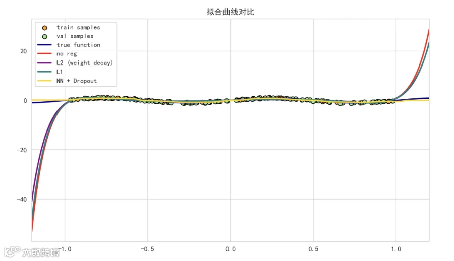
拟合曲线对比:
展示不同方法在整个输入区间上的拟合函数。
-
“无正则化”通常在训练点附近震荡严重,尤其在区间外或数据稀疏处偏离真实函数(明显高方差)。 -
“L2”曲线更平滑,幅度受控,避免了高阶振荡,泛化通常变好。 -
“L1”在某些系数被压成零后,模型可能变得像低阶多项式,曲线更简单甚至有局部平直。 -
“NN + Dropout”作为非线性模型,能拟合复杂形态但 Dropout 帮助减少过拟合,曲线通常更稳定。
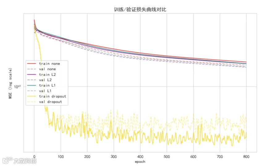
训练/验证损失曲线:
训练损失与验证损失随 epoch 的变化,以 log 纵轴更容易看清数量级差异。
-
无正则化:训练损失会持续下降,但验证损失在达到某个点后回升(过拟合)。 -
L2/L1/Dropout:验证损失更早稳定或更低,说明泛化能力更好。 -
Early stopping:如果看到验证损失在某一轮后上升,就可以借此实施早停策略。
权重分布直方图:
展示模型参数的数值分布。

-
L2 会把权重推向 0 附近,但多数权重仍为小幅连续值(分布窄而高)。 -
L1 会倾向把许多权重变成严格的 0(稀疏)。直方图会显示更多集中在 0 的频率。 -
无正则:权重分布通常更宽、更分散,出现一些大系数,可能导致模型不稳定。
验证误差 vs 正则强度:
展示模型泛化性能如何依赖正则化强度 。

-
通常存在“U 型”曲线:当 很小或为 0 时过拟合(高方差),当 太大时欠拟合(高偏差)。中间有个最优值平衡偏差与方差。 -
该图是调参的重要依据:帮助我们选择合适的正则化强度。
数学上,我们经常把带 L2 的目标写作:
其中 。当使用优化器里的 weight_decay 时,PyTorch 在参数更新时会隐含地做类似于 L2 的收敛控制,所以我们把它当作 L2 正则化来用。L1 则是
,会促使很多 变为 0,得到稀疏权重。
Dropout 的直观解释是:训练时随机丢掉神经元,相当于在训练阶段对许多不同的子网络做平均,从而在测试阶段得到更稳健的预测。它并不直接把权重变小(不像 L2),而是通过 ensemble-like 的效果减少过拟合。
总结
正则化并不是万能药:数据量大且模型合适时,可能不需要强力正则化;反之当模型过于复杂或数据稀少时,正则化很关键。
另外,L2 是“普适且稳妥”的选择(使权重小,模型平滑),通常作为首选;L1 适合希望得到稀疏解或做特征选择时使用;Dropout 更适合大型神经网络。
选择正则化强度 很重要:常用交叉验证或验证集做网格搜索(如上文“验证误差随正则强度的变化”图)。
结合早停、数据增强、减小模型复杂度等手段,通常能取得更好效果。