


哈喽,大家好~
最近有同学留言,数据明明是一条曲线,线性回归怎么都拟合不好,怎么办?
我的建议是,别急着换复杂模型,先给线性回归加几个高次项试试看~
今儿趁这个机会聊聊多项式回归。它适合处理输入与目标之间存在非线性关系,但整体变化仍比较平滑的场景~
多项式回归
普通线性回归只能拟合直线:
如果数据是一条弯曲的趋势线,直线就会出现明显的欠拟合。
多项式回归的做法很直接:给原始特征增加平方项、立方项等高次特征。
其中, 表示多项式阶数, 是截距, 是模型需要学习的参数。
例如,当 、 时,原始数据会被转换成 。模型再对这些新特征做线性组合,就能拟合曲线。
一句话概括:多项式回归不是换了一个全新的回归器,而是先扩展特征,再进行线性回归。
核心原理
虽然 、 看起来是非线性的,但模型对参数 仍然是线性的,所以依旧可以使用线性回归的方法训练。
不过,阶数越高,特征数越多,模型也越容易为了迎合训练数据而发生剧烈弯曲,这就是过拟合。
我们这里使用Ridge回归增加正则化约束:
前半部分要求预测误差尽量小,后半部分限制参数不要过大。 越大,曲线越平滑; 越小,模型越接近普通多项式回归。
Python完整案例
下面生成一组带噪声的三次函数数据,然后比较不同阶数的表现~
import numpy as np
import matplotlib.pyplot as plt
from sklearn.model_selection import train_test_split, KFold, cross_val_score
from sklearn.preprocessing import PolynomialFeatures, StandardScaler
from sklearn.pipeline import make_pipeline
from sklearn.linear_model import Ridge
from sklearn.metrics import mean_squared_error

np.random.seed(42)

# 1. 数据集:真实关系为三次曲线
X = np.random.uniform(-3, 3, 160).reshape(-1, 1)
true_y = 1.5 + 0.8*X[:, 0] - 0.6*X[:, 0]**2 + 0.15*X[:, 0]**3
noise = np.random.normal(0, 0.35 + 0.12*np.abs(X[:, 0]))
y = true_y + noise

X_train, X_test, y_train, y_test = train_test_split(
    X, y, test_size=0.3, random_state=10
)

def build_model(degree):
    return make_pipeline(
        PolynomialFeatures(degree=degree, include_bias=False),
        StandardScaler(),
        Ridge(alpha=0.05)
    )

# 2. 比较1阶、3阶和10阶模型
degrees = [1, 3, 10]
colors = ["#00BFFF", "#FF1493", "#7CFC00"]
models = {}

x_grid = np.linspace(-3, 3, 500).reshape(-1, 1)
true_grid = (1.5 + 0.8*x_grid[:, 0]
             - 0.6*x_grid[:, 0]**2
             + 0.15*x_grid[:, 0]**3)

fig, axes = plt.subplots(1, 2, figsize=(14, 5))

axes[0].scatter(X_train, y_train, s=28, c="#FF8C00",
                alpha=0.7, label="Train data")
axes[0].plot(x_grid, true_grid, "k--", lw=3, label="True curve")

for degree, color in zip(degrees, colors):
    model = build_model(degree)
    model.fit(X_train, y_train)
    models[degree] = model
    axes[0].plot(x_grid, model.predict(x_grid), color=color,
                 lw=2.5, label=f"Degree {degree}")

axes[0].set_title("Polynomial Fitting Comparison")
axes[0].set_xlabel("X")
axes[0].set_ylabel("y")
axes[0].legend()

# 3阶模型的残差分析
model3 = models[3]
train_pred = model3.predict(X_train)
test_pred = model3.predict(X_test)

axes[1].scatter(train_pred, y_train-train_pred, c="#8A2BE2",
                s=35, alpha=0.7, label="Train residual")
axes[1].scatter(test_pred, y_test-test_pred, c="#00CED1",
                s=45, alpha=0.8, label="Test residual")
axes[1].axhline(0, color="#FF4500", lw=2, linestyle="--")
axes[1].set_title("Degree 3 Residual Analysis")
axes[1].set_xlabel("Predicted value")
axes[1].set_ylabel("Residual")
axes[1].legend()

plt.tight_layout()
plt.show()

# 4. 不同阶数的训练、测试与交叉验证误差
degree_range = range(1, 13)
train_rmse, test_rmse, cv_mean, cv_std = [], [], [], []
cv = KFold(n_splits=5, shuffle=True, random_state=42)

for degree in degree_range:
    model = build_model(degree)
    model.fit(X_train, y_train)

    train_rmse.append(mean_squared_error(
        y_train, model.predict(X_train)) ** 0.5)
    test_rmse.append(mean_squared_error(
        y_test, model.predict(X_test)) ** 0.5)

    scores = -cross_val_score(
        build_model(degree), X_train, y_train,
        cv=cv, scoring="neg_root_mean_squared_error"
    )
    cv_mean.append(scores.mean())
    cv_std.append(scores.std())

cv_mean, cv_std = np.array(cv_mean), np.array(cv_std)
best_degree = list(degree_range)[np.argmin(cv_mean)]

plt.figure(figsize=(10, 5))
plt.plot(degree_range, train_rmse, "o-", color="#00BFFF",
         lw=2.5, label="Train RMSE")
plt.plot(degree_range, test_rmse, "s-", color="#FF1493",
         lw=2.5, label="Test RMSE")
plt.plot(degree_range, cv_mean, "^-", color="#7CFC00",
         lw=2.5, label="5-fold CV RMSE")
plt.fill_between(degree_range, cv_mean-cv_std, cv_mean+cv_std,
                 color="#7CFC00", alpha=0.2)
plt.axvline(best_degree, color="#FF8C00", linestyle="--",
            label=f"Best degree = {best_degree}")
plt.xlabel("Polynomial degree")
plt.ylabel("RMSE")
plt.title("Model Complexity and Generalization Error")
plt.xticks(list(degree_range))
plt.legend()
plt.tight_layout()
plt.show()

print("最优阶数:", best_degree)
print("三阶模型测试集RMSE:",
      round(mean_squared_error(y_test, test_pred) ** 0.5, 4))

第一张图左侧比较了1阶、3阶和10阶模型。1阶模型只能画直线,无法捕捉弯曲趋势;3阶模型能还原数据的主要规律;10阶模型更灵活,也更容易追着噪声跑。
右侧是3阶模型的残差图。残差就是 。如果散点随机分布在零线附近,说明模型没有明显遗漏某种变化规律;如果残差呈弧线或漏斗形,就要检查阶数、异常值或噪声结构。
第二张图把阶数与RMSE放在一起。训练误差通常会随着阶
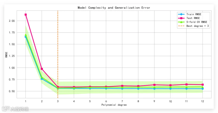
数增加而下降,但测试误差和交叉验证误差会先下降、再上升。最低点对应更合适的模型复杂度,绿色阴影则表示不同折之间的误差波动。
多项式阶数不是越高越好。实际项目中,可以从2到5阶开始,通过交叉验证选择阶数。
高次项的数值范围差异很大,所以特征缩放很重要。我们这里把PolynomialFeatures、StandardScaler和Ridge放进Pipeline,也避免了交叉验证时的数据泄漏。
如果特征数量很多,还要谨慎使用多项式扩展。因为除了平方项,还会产生大量交互项,内存和计算量都会快速增长。
总结
多项式回归的核心,就是把 扩展成 、 等新特征,让线性模型拥有拟合曲线的能力。真正需要控制的不是“能不能拟合”,而是阶数和正则化强度是否合适。
接下来大家可以尝试调整degree和alpha,观察曲线如何变化;也可以把虚拟数据换成房价、销量或温度数据,再通过交叉验证寻找更合适的模型复杂度~