


哈喽,大家好~
今儿和大家来聊聊AdaBoost。
这里,举一个很简单的例子:
比如说你是班级里的老师,要把学生分成两类(比如“优秀”和“不优秀”)。
你请了许多不同的短时间观察员(弱分类器),每个观察员只能做一个很简单的判断(比如“若数学成绩>60 就判为优秀”),这些单一判断可能不准确。
AdaBoost 的思路是:
-
不改观察员的内部能力(不能让弱分类器变强),但允许老师为每个观察员分配一个“话语权”(权重)。
-
数据集中每个样本在训练过程中会带有一个“被关注程度”(样本权重)。一开始,所有样本被同等对待。
-
每轮训练:训练一个弱分类器,让它尽可能在当前样本权重下做好分类(重点关注高权重样本)。算出它的错误率 (按样本权重算),然后给这个弱分类器分配一个权重 ,错误率低的观察员权重更高。
-
更新样本权重:把被当前弱分类器错误分类的样本权重提高,正确分类的样本权重降低。这样下一轮训练时,新的弱分类器会“更关注”之前被错分的样本。
-
重复多轮,最后将所有弱分类器按其权重 加权投票(或线性组合),得到最终强分类器。
数学上,常见形式的权重 和样本权重更新为:
-
弱分类器在第 轮的加权错误率
-
弱分类器权重
-
样本权重更新(未归一化)
其中 , 。更新后需归一化使 。
最终强分类器为
为什么它有效?直觉上来说,每轮都在减少训练集中加权错误,最终训练误差会呈指数下降(理论上),同时通过集成不同简单规律,能学习到复杂的决策边界。
实战案例
我们这里生成二维数据,两类非线性分布,用决策树桩作为弱分类器实现 AdaBoost。
代码中注释非常的详细,大家可以按照步骤来逐步学习~
import torch
import numpy as np
import matplotlib.pyplot as plt
from matplotlib.colors import ListedColormap

torch.manual_seed(0)
np.random.seed(0)

# 1. 两类、非线性混合
def make_toy_data(n=300):
    # 类别1:两个环的一部分
    r1 = 1.0 + 0.4 * np.random.randn(n//3)
    theta1 = np.random.uniform(0, 2*np.pi, n//3)
    x1 = np.stack([r1 * np.cos(theta1), r1 * np.sin(theta1)], axis=1)

    r2 = 2.5 + 0.4 * np.random.randn(n//3)
    theta2 = np.random.uniform(0, 2*np.pi, n//3)
    x2 = np.stack([r2 * np.cos(theta2), r2 * np.sin(theta2)], axis=1)

    # 类别2:椭圆/云
    x3 = np.random.randn(n - 2*(n//3), 2) * 0.6 + np.array([1.0, -1.2])

    X = np.vstack([x1, x2, x3])
    y = np.hstack([np.ones(x1.shape[0]), np.ones(x2.shape[0]), -np.ones(x3.shape[0])])
    return X.astype(np.float32), y.astype(np.int64)

X_np, y_np = make_toy_data(300)
X = torch.tensor(X_np)
y = torch.tensor(y_np, dtype=torch.float32)  # +1 / -1

# 2. 决策桩弱分类器
class DecisionStumpTorch:
    def __init__(self):
        self.feature_idx = None
        self.threshold = None
        self.polarity = 1# 1 or -1

    def fit(self, X, y, sample_weights):
        # X: (n, d), y: (n,), sample_weights: (n,)
        n, d = X.shape
        best_error = float('inf')
        best = None

        for feat in range(d):
            x_feat = X[:, feat]
            sorted_vals, idx = torch.sort(x_feat)
            # candidate thresholds: midpoints between consecutive values
            thresholds = (sorted_vals[:-1] + sorted_vals[1:]) / 2.0
            thresholds = torch.unique(thresholds)
            # Also consider thresholds slightly below min and above max
            thresholds = torch.cat([thresholds, sorted_vals[:1] - 1e-3, sorted_vals[-1:] + 1e-3])

            for thr in thresholds:
                for polarity in [1, -1]:
                    # prediction: polarity * sign(x_feat - thr)
                    preds = torch.ones_like(y)
                    preds[polarity * (x_feat - thr) < 0] = -1
                    # weighted error
                    err = torch.sum(sample_weights * (preds != y).float()).item()
                    if err < best_error:
                        best_error = err
                        best = (feat, float(thr), int(polarity), preds.clone())
        if best isNone:
            # fallback
            self.feature_idx, self.threshold, self.polarity = 0, 0.0, 1
        else:
            self.feature_idx, self.threshold, self.polarity = best[0], best[1], best[2]
        return best_error

    def predict(self, X):
        x_feat = X[:, self.feature_idx]
        preds = torch.ones(X.shape[0], dtype=torch.float32)
        preds[self.polarity * (x_feat - self.threshold) < 0] = -1.0
        return preds

# 3. AdaBoost 训练
def train_adaboost(X, y, T=20):
    n = X.shape[0]
    D = torch.ones(n, dtype=torch.float32) / n  # sample weights
    stumps = []
    alphas = []
    train_errors = []
    Zs = []

    for t in range(T):
        stump = DecisionStumpTorch()
        err = stump.fit(X, y, D)  # weighted error
        # numerical stability
        err = min(max(err, 1e-10), 1 - 1e-10)
        alpha = 0.5 * math.log((1 - err) / err)
        preds = stump.predict(X)
        # update D
        D = D * torch.exp(-alpha * y * preds)
        Z = torch.sum(D).item()
        D = D / Z

        # store
        stumps.append(stump)
        alphas.append(alpha)
        Zs.append(Z)
        # compute cumulative train error
        agg = torch.zeros(n)
        for a, s in zip(alphas, stumps):
            agg += a * s.predict(X)
        agg_preds = torch.sign(agg)
        train_err = torch.mean((agg_preds != y).float()).item()
        train_errors.append(train_err)

        # print progress
        # print(f"Iter {t+1}: err={err:.4f}, alpha={alpha:.4f}, train_err={train_err:.4f}")
    return stumps, alphas, train_errors, Zs, D

stumps, alphas, train_errors, Zs, final_D = train_adaboost(X, y, T=20)

# 4. 可视化函数
def plot_dataset_weights(X, y, weights, ax):
    # weights scaled for plotting sizes
    sizes = 50 + (weights.numpy() - weights.min().item()) / (weights.max().item() - weights.min().item() + 1e-12) * 400
    colors = np.where(y.numpy() > 0, 'tab:orange', 'tab:purple')
    ax.scatter(X[:,0], X[:,1], s=sizes, c=colors, edgecolors='k', alpha=0.85)
    ax.set_title("样本数据(点大小=样本权重)")
    ax.set_xlabel("x1"); ax.set_ylabel("x2")

def plot_stump_decision(stump, ax, title):
    # plot decision boundary for one stump
    xx, yy = np.meshgrid(np.linspace(X_np[:,0].min()-0.5, X_np[:,0].max()+0.5, 300),
                         np.linspace(X_np[:,1].min()-0.5, X_np[:,1].max()+0.5, 300))
    grid = torch.tensor(np.c_[xx.ravel(), yy.ravel()], dtype=torch.float32)
    preds = stump.predict(grid).numpy().reshape(xx.shape)
    cmap = ListedColormap(['#ffcccc', '#cce5ff'])
    ax.contourf(xx, yy, preds, cmap=cmap, alpha=0.8, levels=[-1,0,1])
    # scatter data
    colors = np.where(y_np > 0, 'tab:orange', 'tab:purple')
    ax.scatter(X_np[:,0], X_np[:,1], c=colors, edgecolors='k')
    ax.set_title(title)

def plot_ensemble_boundary(stumps, alphas, ax, title):
    xx, yy = np.meshgrid(np.linspace(X_np[:,0].min()-0.5, X_np[:,0].max()+0.5, 400),
                         np.linspace(X_np[:,1].min()-0.5, X_np[:,1].max()+0.5, 400))
    grid = torch.tensor(np.c_[xx.ravel(), yy.ravel()], dtype=torch.float32)
    agg = torch.zeros(grid.shape[0])
    for a, s in zip(alphas, stumps):
        agg += a * s.predict(grid)
    preds = torch.sign(agg).numpy().reshape(xx.shape)
    cmap = plt.cm.seismic
    ax.contourf(xx, yy, preds, levels=1, cmap=cmap, alpha=0.6)
    colors = np.where(y_np > 0, 'tab:orange', 'tab:purple')
    ax.scatter(X_np[:,0], X_np[:,1], c=colors, edgecolors='k')
    ax.set_title(title)

# 5. 可视化
fig, axes = plt.subplots(2, 3, figsize=(18, 12))
axes = axes.ravel()

# (1) 初始样本与初始权重(相等)
plot_dataset_weights(X, y, torch.ones(X.shape[0]) / X.shape[0], axes[0])
axes[0].set_title("(1) 初始样本(权重均等)")

# (2) 第 1 个弱分类器边界
plot_stump_decision(stumps[0], axes[1], "(2) 第 1 个弱分类器(stump)")

# (3) 第 5 个弱分类器边界(观察不同弱分类器)
plot_stump_decision(stumps[4], axes[2], "(3) 第 5 个弱分类器(stump)")

# (4) 随训练轮数的训练误差变化 & Z(归一化常数)变化
axes[3].plot(range(1, len(train_errors)+1), train_errors, marker='o', color='tab:blue', label='训练错误率')
axes[3].set_xlabel("迭代轮数")
axes[3].set_ylabel("训练错误率")
axes[3].set_ylim(0, 1)
axes[3].grid(True)
axes[3].set_title("(4) 训练错误率随迭代变化")
axes_twin = axes[3].twinx()
axes_twin.plot(range(1, len(Zs)+1), Zs, marker='s', color='tab:orange', label='Z_t (归一化常数)')
axes_twin.set_ylabel("Z_t")
axes_twin.legend(loc='upper right')

# (5) 最终集成的决策边界
plot_ensemble_boundary(stumps, alphas, axes[4], "(5) 最终 AdaBoost 集成决策边界")

# (6) margin 分布(直方图)
# margin = y * sum alpha * h(x)
agg_on_train = torch.zeros(X.shape[0])
for a, s in zip(alphas, stumps):
    agg_on_train += a * s.predict(X)
margins = (y * agg_on_train).numpy()
axes[5].hist(margins, bins=30, color='tab:green', edgecolor='k', alpha=0.9)
axes[5].axvline(0, color='red', linestyle='--', label='margin=0')
axes[5].set_title("(6) margin 分布(y * sum alpha*h(x))")
axes[5].set_xlabel("margin 值")
axes[5].set_ylabel("样本数")
axes[5].legend()

plt.tight_layout()
plt.show()

# 额外绘图:样本权重随迭代变化(热力图或散点大小随迭代)
# 将每轮的样本权重保存在训练函数中,可以改造上面 train_adaboost 来记录更多数据。
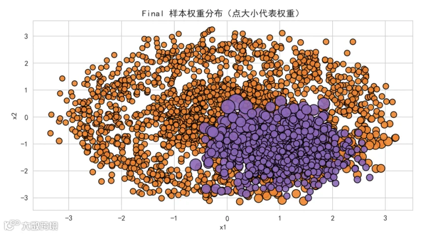
# 为简洁,下面演示如何绘制最终权重大小的空间分布(点大小为 final_D)
plt.figure(figsize=(6,5))
sizes = 50 + (final_D.numpy() - final_D.min().item()) / (final_D.max().item() - final_D.min().item() + 1e-12) * 400
colors = np.where(y_np > 0, 'tab:orange', 'tab:purple')
plt.scatter(X_np[:,0], X_np[:,1], s=sizes, c=colors, edgecolors='k', alpha=0.9)
plt.title("Final 样本权重分布(点大小代表权重)")
plt.xlabel("x1"); plt.ylabel("x2")
plt.show()
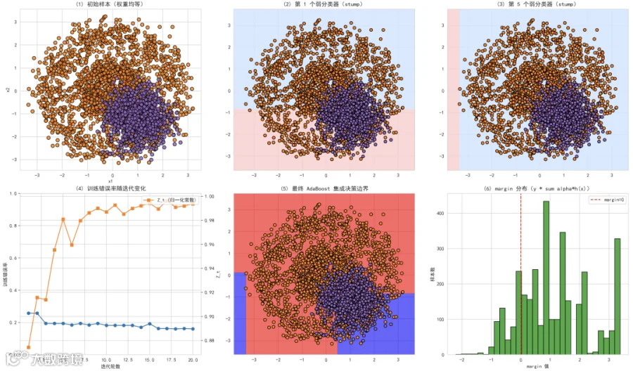
初始数据(点大小=样本权重):
展示训练集初始的分布与类标签。这里初始权重均等,所以点大小一致。
可以直观看出数据是否线性可分、是否存在明显的类别重叠,这对随后理解弱分类器的作用有帮助。
第 1 轮和第 5 轮弱分类器的决策边界:
决策桩只根据一个特征与一个阈值进行划分,边界通常是直线(垂直于某一坐标轴)。
通过查看不同轮的弱分类器边界,可以理解 AdaBoost 是如何“聚焦到难样本”并产生不同的弱分类器。
训练误差随迭代变化 & Z_t(归一化常数):
训练误差(集成前 t 轮的加权投票后错误率)通常随着迭代减少;Z_t 是权重更新的归一化常数,它与误差有关。
AdaBoost 最小化了训练集的指数损失,训练误差可以以指数速度下降(在理想条件下)。
最终 AdaBoost 集成决策边界:
展示集成后的强分类器决策边界。通常比单个弱分类器复杂很多,能抓住非线性边界。
-
观察边界是否能把两类区分开; -
看边界是否对局部噪声过度弯曲(过拟合的迹象)。
margin 分布(y * sum alpha*h(x)):
每个样本的 margin 定义为 ,反映了模型对样本分类的“置信度”。margin 为正且大,表示分类且置信;margin 负值则表示被错误分类。
-
margin 分布右移(更多正值且较大)表示模型对样本更有信心; -
若许多样本 margin 接近 0,说明这些样本处在决策边界附近,是难分类样本; -
若少数样本 margin 很小或为负,可能是噪声或异常点。
实验中的注意事项
弱分类器的选择:
决策桩适合教学和演示;工业中常用浅层决策树(如 max_depth=1/2/3)或其他弱学习器。
迭代次数 :
过少可能学习不足,过多可能在存在噪音的情况下过拟合。通常通过交叉验证选择 。
噪音和离群点:
AdaBoost 在存在标签噪音时可能把注意力过多放在这些噪音点上,导致过拟合。可改用基于样本裁剪或调整 loss 的变种(如 AdaBoost.R2、SAMME.R、Regularized Boosting)。
可扩展性:
纯 Python/单机实现适合教学,工业中可用 XGBoost、LightGBM、CatBoost 等高性能库(基于梯度提升树,不是 AdaBoost,但思想相近:集合多棵树)。
PyTorch 与 sklearn:
我们用 PyTorch 做张量运算展示,实际可直接用 sklearn.ensemble.AdaBoostClassifier 快速尝试。
总结
AdaBoost 它的关键在于“给错了的样本更多关注”,并把训练好的弱分类器按表现给予不同的话语权(权重)。
最终把这些弱观察员加起来后,整体可以做出很强的判断。