




@白露未晞me
开源项目《Games》 作者
原问题:深度学习里有哪些神奇有趣的现象?
谢邀。笑死,我来歪个楼,讲几个没那么「正经」的现象。
NO.1
Understanding Deep Learning Requires Rethinking Generalization
16 年的论文,现在差不多 6-7k 的 citations 了,算是深度学习泛化理论里一个很经典的反直觉结果。比如把二维点完全随机分成红蓝两类:位置和类别没有任何关系。足够大的神经网络仍然可以把训练集硬背下来,很好地拟合随机标签,这也是为什么「训练误差低」本身完全不能解释泛化。
( 2026 年 8 月 26 日补充:貌似有一些评论对此有异议,展开聊一下吧。
现在看当然不算特别反直觉,但这是拿今天的常识倒推 2016 年。而且我怀疑很多人本身就理解错重点了,而不是是不是用现代视角看的问题,这篇论文真正冲击的并不是「神经网络居然能记住训练集」,而是同一个网络明明有能力把完全随机的标签都拟合到零误差,为什么在真实标签上训练时却又能很好地泛化? 在此之前我们很容易把「不会过拟合」理解成「模型没能力乱背」;而这篇论文告诉你这是不对的,模型完全有能力乱背。于是问题就变成了:既然它能乱背,为什么真实世界里却常常没有乱背? 这也说明,仅靠「限制模型容量、通过正则化避免过拟合」这套传统直觉,并不足以解释现代深度网络的泛化。这篇论文的重要性,就是把这个矛盾用一个非常直接的实验摆了出来;后来 implicit bias、margin/norm-based explanations、double descent 等大量工作,其实都在从不同角度继续回答这个问题。)
一个非常简单的复现代码如下:
import torchimport torch.nn as nnimport matplotlib.pyplot as pltimport numpy as nptorch.manual_seed(0)N = 200X = torch.rand(N, 2) * 2 - 1# 完全随机标签y = torch.randint(0, 2, (N,))net = nn.Sequential(nn.Linear(2, 128), nn.ReLU(),nn.Linear(128, 128), nn.ReLU(),nn.Linear(128, 128), nn.ReLU(),nn.Linear(128, 2))opt = torch.optim.Adam(net.parameters(), lr=2e-3)loss_fn = nn.CrossEntropyLoss()a = np.linspace(-1, 1, 150)gx, gy = np.meshgrid(a, a)grid = torch.tensor(np.c_[gx.ravel(), gy.ravel()],dtype=torch.float32)plt.ion()fig, ax = plt.subplots()for step inrange(4000):out = net(X)loss = loss_fn(out, y)opt.zero_grad()loss.backward()opt.step()if step % 50 == 0:with torch.no_grad():z = net(grid).softmax(1)[:, 1]z = z.reshape(150, 150)acc = (net(X).argmax(1) == y).float().mean()ax.clear()ax.contourf(gx, gy, z,levels=np.linspace(0, 1, 15),alpha=0.7)ax.scatter(X[:, 0], X[:, 1],c=y,edgecolors="black")ax.set_title(f"step={step}, train acc={acc:.3f}")plt.pause(0.001)plt.ioff()plt.show()
效果大概长这样,最后 acc 基本都能到 100%:
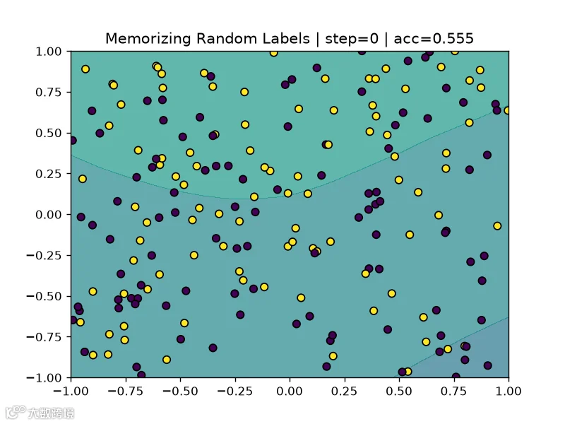
Understanding Deep Learning Requires Rethinking Generalization
NO. 2
On the Spectral Bias of Neural Networks
也是一篇几千 citations 的论文 Orz,核心发现是 spectral bias。即不同频率具有不同学习速度。
比如你设目标函数 f(x)= \sin x+0.3\sin(10x). 明明两部分同时存在,但 MLP 通常会先把低频的 \sin x 学出来,然后高频小波纹才慢慢出现。
一个简单的复现代码如下:
import torchimport torch.nn as nnimport matplotlib.pyplot as pltimport mathimport numpy as npimport imageio.v2 as imageiotorch.manual_seed(0)x = torch.linspace(-math.pi, math.pi, 500)[:, None]low = torch.sin(x)high = 0.3 * torch.sin(10 * x)y = low + highnet = nn.Sequential(nn.Linear(1, 128), nn.Tanh(),nn.Linear(128, 128), nn.Tanh(),nn.Linear(128, 1))opt = torch.optim.Adam(net.parameters(), lr=1e-3)plt.ion()fig, ax = plt.subplots()ax.plot(x, y, label="target", linewidth=2)line, = ax.plot(x, torch.zeros_like(x), label="network", linewidth=2)ax.set_xlim(-math.pi, math.pi)ax.set_ylim(-1.6, 1.6)ax.legend()frames = []for step inrange(10001):pred = net(x)loss = ((pred - y) ** 2).mean()opt.zero_grad()loss.backward()opt.step()# 前面变化快,多保存;后面变化慢,少保存save_frame = ((step < 2000and step % 20 == 0)or(2000 <= step < 6000and step % 50 == 0)or(step >= 6000and step % 100 == 0))if save_frame:with torch.no_grad():pred = net(x)line.set_ydata(pred.numpy())ax.set_title(f"Spectral Bias | step={step} | loss={loss.item():.5f}")plt.pause(0.001)fig.canvas.draw()frame = np.asarray(fig.canvas.buffer_rgba())[:, :, :3].copy()frames.append(frame)plt.ioff()imageio.mimsave("spectral_bias.gif",frames,duration=0.05,loop=0)plt.show()
效果如下:

On the Spectral Bias of Neural Networks
NO.3
The Large Learning Rate Phase of Deep Learning: the Catapult Mechanism
这篇论文目前大概几百的 citations,它描述了一个很有意思的现象。
我们的传统直觉是:学习率太大 → loss 爆炸 → 训练废了。
但神经网络有一个相当奇怪的区域:loss 可以突然暴涨几十、几百甚至几千倍,之后重新跌下来继续正常训练。Lewkowycz 等人把这类大步长动力学称为 catapult mechanism;后续也有类似工作观察到 SGD 中明显的 loss spike,并研究了其与 feature learning 的关系:
Catapults in SGD: spikes in the training loss and their impact on generalization through feature learning
这篇论文的复现也十分方便,代码如下:
import torchimport torch.nn as nnimport matplotlib.pyplot as pltimport numpy as npimport imageio.v2 as imageiotorch.manual_seed(0)torch.set_num_threads(1)x = torch.linspace(-1, 1, 256)[:, None]y = torch.sin(5 * x)net = nn.Sequential(nn.Linear(1, 256),nn.ReLU(),nn.Linear(256, 1))opt = torch.optim.SGD(net.parameters(), lr=0.05)history = []plt.ion()fig, ax = plt.subplots(figsize=(8, 5))line, = ax.plot([], [])ax.set_yscale("log")ax.set_xlim(0, 300)ax.set_ylim(0.25, 2000)ax.set_xlabel("step")ax.set_ylabel("loss")ax.set_title("step=0, loss=0")ax.grid(alpha=0.25)fig.tight_layout()plt.show(block=False)with imageio.get_writer("training.gif", mode="I", fps=20, loop=0) as writer:for step inrange(300):pred = net(x)loss = ((pred - y) ** 2).mean()opt.zero_grad()loss.backward()opt.step()history.append(loss.item())line.set_data(range(len(history)), history)ax.set_title(f"step={step}, loss={loss.item():.3g}")fig.canvas.draw()fig.canvas.flush_events()frame = np.asarray(fig.canvas.buffer_rgba())[..., :3].copy()writer.append_data(frame)plt.pause(0.02)plt.ioff()plt.show()
效果如下:
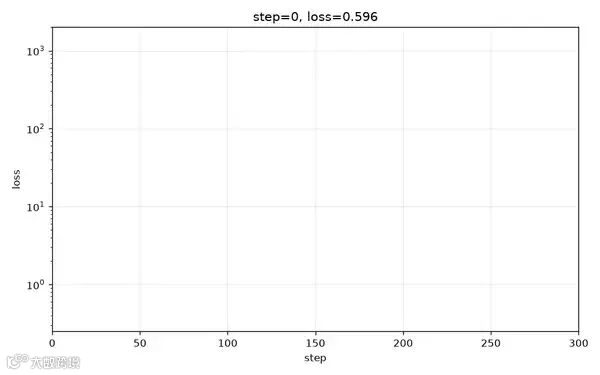
The Large Learning Rate Phase of Deep Learning: the Catapult Mechanism
NO.4
Grokking: Generalization Beyond Overfitting on Small Algorithmic Datasets
这也是一篇小 1k citations 的论文,这篇论文大概说了这么一件事。
让模型学习: 模型训练的 accuracy 很快就能达到 100%,但 test accuracy 可能长期接近随机,然后经过大量额外训练才明显上升。
Power 等人的原始工作把这种「过拟合很久之后才出现泛化」称为 grokking。
复现代码如下:
import torchimport torch.nn as nnimport matplotlib.pyplot as pltfrom matplotlib.animation import PillowWritertorch.manual_seed(0)torch.set_num_threads(1)p = 23X = torch.cartesian_prod(torch.arange(p),torch.arange(p))y = (X[:, 0] + X[:, 1]) % pperm = torch.randperm(len(X))n_train = len(X) // 2train = perm[:n_train]test = perm[n_train:]classModel(nn.Module):def__init__(self):super().__init__()self.emb = nn.Embedding(p, 16)self.mlp = nn.Sequential(nn.Linear(32, 64),nn.ReLU(),nn.Linear(64, p))defforward(self, x):a = self.emb(x[:, 0])b = self.emb(x[:, 1])return self.mlp(torch.cat([a, b], dim=1))net = Model()opt = torch.optim.AdamW(net.parameters(),lr=3e-3,weight_decay=1.0)loss_fn = nn.CrossEntropyLoss()train_hist = []test_hist = []steps = []plt.ion()fig, ax = plt.subplots()l1, = ax.plot([], [], label="train")l2, = ax.plot([], [], label="test")ax.set_ylim(0, 1.05)ax.legend()# 新增:GIF writerwriter = PillowWriter(fps=10)# 新增:保存 GIFwith writer.saving(fig, "grokking.gif", dpi=100):for step inrange(15000):out = net(X[train])loss = loss_fn(out,y[train])opt.zero_grad()loss.backward()opt.step()if step % 100 == 0:with torch.no_grad():train_acc = (net(X[train]).argmax(1)== y[train]).float().mean()test_acc = (net(X[test]).argmax(1)== y[test]).float().mean()steps.append(step)train_hist.append(train_acc)test_hist.append(test_acc)l1.set_data(steps, train_hist)l2.set_data(steps, test_hist)ax.relim()ax.autoscale_view(scalex=True, scaley=False)ax.set_title(f"step={step} "f"train={train_acc:.2f} "f"test={test_acc:.2f}")plt.pause(0.001)# 新增:把当前画面写入 GIFwriter.grab_frame()plt.ioff()plt.show()
效果如下:
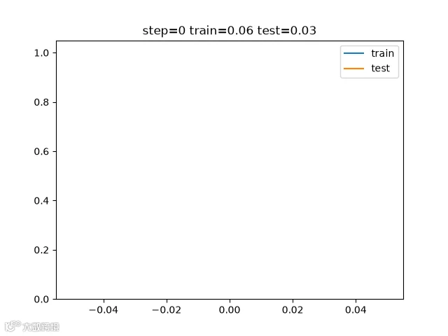
Grokking: Generalization Beyond Overfitting on Small Algorithmic Datasets
NO. 5 Toy Models of Superposition
差不多也是一篇小 1k citations 的论文。
Superposition 指的是:当模型的表示维度小于潜在特征数量时,网络并不一定为每个特征分配独立的神经元或维度,而可能让多个特征共享同一个表示空间。尤其当特征是稀疏激活的、很少同时出现时,这种「叠加存储」可以显著提高有限表示容量的利用率。代价是不同特征之间会产生一定干扰。Elhage 等人系统展示了这一现象,并发现模型会自发形成具有几何结构的特征表示。
简单复现一下:
import torchimport matplotlib.pyplot as pltfrom matplotlib.animation import PillowWritertorch.manual_seed(0)torch.set_num_threads(1)features = 5hidden = 2# 每个 feature 在二维隐藏空间里的方向W = torch.nn.Parameter(torch.randn(hidden, features) * 0.2)b = torch.nn.Parameter(torch.zeros(features))opt = torch.optim.Adam([W, b],lr=3e-3)plt.ion()fig, ax = plt.subplots(figsize=(5, 5))writer = PillowWriter(fps=10)with writer.saving(fig, "superposition.gif", dpi=100):for step inrange(8000):# sparse featuresx = torch.rand(1024, features)mask = (torch.rand_like(x) > 0.9).float()x = x * mask# compress 5D -> 2Dh = x @ W.T# reconstructy = torch.relu(h @ W + b)loss = ((y - x) ** 2).mean()opt.zero_grad()loss.backward()opt.step()if step % 100 == 0:ax.clear()w = W.detach()for i inrange(features):ax.arrow(0, 0,w[0, i],w[1, i],head_width=0.05,length_includes_head=True)ax.text(w[0, i] * 1.1,w[1, i] * 1.1,str(i))ax.set_xlim(-1.5, 1.5)ax.set_ylim(-1.5, 1.5)ax.set_aspect("equal")ax.set_title(f"step={step}, loss={loss.item():.4f}")plt.pause(0.01)writer.grab_frame()plt.ioff()plt.show()
效果如下:

Toy Models of Superposition
NO. 6 Deep Image Prior
这篇论文感觉做 cv 的应该都知道。
它的核心发现是:即使 CNN 完全没有经过训练,它的网络结构本身也天然偏向生成自然、平滑且具有局部结构的图像。 因此,只需固定一份随机噪声作为输入,用单张受损或含噪图像反向优化网络参数,CNN 往往会先拟合出图像中的真实结构,再逐渐拟合噪声。这个现象说明,网络架构本身就可以充当一种有效的图像先验,而不一定依赖大规模训练数据。
一个简单的测试代码:
import torchimport torch.nn as nnimport torch.nn.functional as Fimport matplotlib.pyplot as pltfrom matplotlib.animation import PillowWritertorch.manual_seed(0)torch.set_num_threads(1)H = W = 64yy, xx = torch.meshgrid(torch.linspace(-1, 1, H),torch.linspace(-1, 1, W),indexing="ij")clean = torch.zeros(H, W)# 圆clean[(xx + 0.35) ** 2+ (yy + 0.15) ** 2< 0.18 ** 2] = 1# 方块clean[(xx > 0.05) &(xx < 0.65) &(yy > -0.5) &(yy < -0.1)] = 0.7clean = clean[None, None]noisy = (clean+ 0.25 * torch.randn_like(clean)).clamp(0, 1)classGenerator(nn.Module):def__init__(self):super().__init__()self.c1 = nn.Conv2d(16, 64, 3, padding=1)self.c2 = nn.Conv2d(64, 64, 3, padding=1)self.c3 = nn.Conv2d(64, 32, 3, padding=1)self.c4 = nn.Conv2d(32, 1, 3, padding=1)defforward(self, z):x = F.relu(self.c1(z))x = F.interpolate(x,scale_factor=2,mode="bilinear")x = F.relu(self.c2(x))x = F.interpolate(x,scale_factor=2,mode="bilinear")x = F.relu(self.c3(x))x = F.interpolate(x,scale_factor=2,mode="bilinear")return torch.sigmoid(self.c4(x))net = Generator()# 固定随机输入z = torch.rand(1, 16, 8, 8)opt = torch.optim.Adam(net.parameters(),lr=5e-3)plt.ion()fig, ax = plt.subplots(1, 3)ax[0].imshow(clean[0, 0],cmap="gray")ax[0].set_title("clean")ax[1].imshow(noisy[0, 0],cmap="gray")ax[1].set_title("noisy")writer = PillowWriter(fps=10)with writer.saving(fig, "deep_image_prior.gif", dpi=100):for step inrange(500):out = net(z)# 注意:网络只看 noisy!loss = ((out - noisy) ** 2).mean()opt.zero_grad()loss.backward()opt.step()if step % 10 == 0:ax[2].clear()ax[2].imshow(out[0, 0].detach(),cmap="gray",vmin=0,vmax=1)ax[2].set_title(f"network step={step}")plt.pause(0.01)writer.grab_frame()plt.ioff()plt.show()
效果如下:
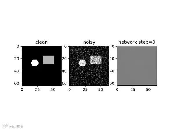
Deep Image Prior
后续看到其他有意思的再补充吧。

知友讨论
@东田鸟:
博主的这篇回答远胜过国内诸多大学ai课…
@我在这里寻宝:
好回答。最后一个我也读过,很有意思哈哈哈,跟现在的各种刷sota的复杂模型对比是一股清流。
@志愿的人:
Deep Image Prior这篇文章的论证我感觉是薄弱的,甚至可以用上面论文的结论来反驳它:On the Spectral Bias of Neural Networks论证了mlp模型是先学习低频信号,再学习高频。图像里的结构信息就是低频,噪声是高频。既然mlp结构就会先学习低频信息,这说明这一现象与CNN结构无关。
@QuinHai:
No1 其实说明了业界主流观点,压缩即智能
示例里面总可训练参数量: 33666
训练样本数量: 200
参数量 / 样本数 = 168.33
而GPT3是175B的参数量,训练Token 300B
下面有压缩即智能的实验研究
Language Modeling Is Compression (2024‑05) arXiv:2405.04762
Compression Represents Intelligence Linearly (COLM 2024) arXiv:2404.09937
阅读更多
🤝 知乎 AI Researcher Club 招募:
知乎联合 10+ 家媒体、创投孵化合作伙伴发起「AI Researcher Club」共创计划,长期支持支持 AI 前沿研究者,让重要的研究被看见、被讨论,让研究者找到彼此,也让新的合作由此发生。点击了解 >> AI Researcher Club
🚀 知乎 AI 社群:
如果你对 AI 共识、AI 活动感兴趣,欢迎扫码加入知乎社群↓,我们将每周送上知乎 AI 周报,分享社区内的 AI 讨论与共识,并不定时送上 AI 各类活动报名。

知乎AI情报站
让一部分开发者先走起来
🚀 知乎科技账号 @ZhihuFrontier 正式登陆 X
👉🏻 https://www.zhihu.com/project-square,上传你的 Vibe Coding 项目,在知乎遇见更多可能。