导师急了：“数据类型没搞懂，直接训练模型？”我：“Codex代码都跑通了！”导师：“字符串转数值、One-Hot编码，这些坑你踩过几个？”

哈喽，大家好~

有同学最近提到，这列明明都是数字，为什么模型还是报错？

很多刚刚接触的同学，都会碰到这样的问题，因为在模型眼里，58和"58岁"完全是两种数据。

项目里的数据，很少能拿来直接训练模型。金额带货币符号、日期格式不统一、布尔值写成“是/否”，这些问题都属于数据类型转换。

数据类型为什么会影响模型

假设收入这一列保存的是：

¥58,000
¥9,500
--

人可以看出前两个是金额，但Python会把整列识别成字符串。此时不仅无法计算均值，也不能直接送进大多数机器学习模型。

数据类型转换，本质上是一个映射过程：

这里 是原始数据， 是清洗规则， 是转换后的标准数据。例如：

如果遇到"--"或者"unknown"，不要强行填成0，而是先转换为缺失值，再通过中位数、众数等方法处理。

也就是说，类型转换不是简单改格式，而是在恢复数据原本的业务含义。

不同类型应该怎么转换

数值字段要先去掉单位、逗号和货币符号，再使用pd.to_numeric()。

日期字段统一转成datetime后，通常还要提取年份、月份或注册天数。

类别字段则不能随便转成整数。比如北京、上海、深圳编码成1、2、3，会让模型误以为深圳“大于”上海。我们这里使用One-Hot编码，避免制造不存在的大小关系。

布尔字段也要统一，例如将“是/否”转换为1和0。

模型原理

案例使用逻辑回归预测客户是否流失。

模型先计算线性得分，再通过Sigmoid函数得到概率：

其中 是清洗后的客户特征， 是模型学习到的权重， 是偏置项。输出越接近1，客户流失风险越高。

逻辑回归结构简单，结果稳定，很适合用来验证数据清洗是否有效。

Python实现

下面咱们构造一份客户数据，故意加入“岁”、货币符号、混合日期和非法字符。

import numpy as np
import pandas as pd
import matplotlib.pyplot as plt

from sklearn.model_selection import train_test_split
from sklearn.compose import ColumnTransformer
from sklearn.pipeline import Pipeline
from sklearn.preprocessing import OneHotEncoder, StandardScaler
from sklearn.impute import SimpleImputer
from sklearn.linear_model import LogisticRegression
from sklearn.metrics import (
    roc_curve, precision_recall_curve,
    roc_auc_score, average_precision_score
)

rng = np.random.default_rng(42)
n = 2500
ref_date = pd.Timestamp("2025-01-01")

# 生成真实变量
age = rng.integers(18, 66, n)
income = rng.lognormal(10.8, 0.45, n)
vip = rng.binomial(1, 0.25, n)
city = rng.choice(["北京", "上海", "深圳", "成都"], n)
days = rng.integers(30, 1000, n)

city_effect = pd.Series(city).map(
    {"北京": 0.2, "上海": 0.35, "深圳": 0.25, "成都": -0.15}
).to_numpy()

score = (-1.2 + 0.045 * (age - 38)
         + 0.000018 * (income - 50000)
         + 0.8 * vip + 0.0012 * days + city_effect)

prob = 1 / (1 + np.exp(-score))
target = rng.binomial(1, prob)

signup = ref_date - pd.to_timedelta(days, unit="D")
date_text = np.array([
    d.strftime("%Y-%m-%d") if i % 3 == 0
    else d.strftime("%Y/%m/%d") if i % 3 == 1
    else d.strftime("%d-%m-%Y")
    for i, d in enumerate(signup)
])

# 制造脏数据
df = pd.DataFrame({
    "age": [f"{x}岁" for x in age],
    "income": [f"¥{x:,.2f}" for x in income],
    "vip": np.where(vip == 1, "是", "否"),
    "city": city,
    "signup_date": date_text,
    "churn": target
})

df.loc[rng.choice(n, 70, replace=False), "age"] = "unknown"
df.loc[rng.choice(n, 55, replace=False), "income"] = "--"
df.loc[rng.choice(n, 45, replace=False), "signup_date"] = "日期错误"
df.loc[rng.choice(n, 30, replace=False), "vip"] = "未知"

# 类型转换
df["age_num"] = pd.to_numeric(
    df["age"].str.extract(r"(\d+)")[0], errors="coerce"
)

df["income_num"] = pd.to_numeric(
    df["income"].str.replace(r"[¥,]", "", regex=True),
    errors="coerce"
)

df["vip_num"] = df["vip"].map({"是": 1, "否": 0})

def parse_date(x):
    for fmt in ("%Y-%m-%d", "%Y/%m/%d", "%d-%m-%Y"):
        try:
            return pd.to_datetime(x, format=fmt)
        except (ValueError, TypeError):
            pass
    return pd.NaT

df["date_num"] = df["signup_date"].apply(parse_date)
df["signup_days"] = (ref_date - df["date_num"]).dt.days

features = ["age_num", "income_num", "vip_num",
            "signup_days", "city"]
X = df[features]
y = df["churn"]

print("转换后的缺失率：")
print(X.isna().mean().round(3))

X_train, X_test, y_train, y_test = train_test_split(
    X, y, test_size=0.3, stratify=y, random_state=42
)

num_cols = ["age_num", "income_num", "vip_num", "signup_days"]
cat_cols = ["city"]

preprocessor = ColumnTransformer([
    ("num", Pipeline([
        ("imputer", SimpleImputer(strategy="median")),
        ("scaler", StandardScaler())
    ]), num_cols),
    ("cat", Pipeline([
        ("imputer", SimpleImputer(strategy="most_frequent")),
        ("onehot", OneHotEncoder(handle_unknown="ignore"))
    ]), cat_cols)
])

model = Pipeline([
    ("clean", preprocessor),
    ("model", LogisticRegression(max_iter=1000))
])

model.fit(X_train, y_train)
pred_prob = model.predict_proba(X_test)[:, 1]

print("ROC-AUC:", round(roc_auc_score(y_test, pred_prob), 3))
print("AP:", round(average_precision_score(y_test, pred_prob), 3))

可视化

继续加入下面的代码，绘制ROC、PR以及不同阈值下的Precision、Recall和F1变化。

fpr, tpr, _ = roc_curve(y_test, pred_prob)
precision, recall, thresholds = precision_recall_curve(
    y_test, pred_prob
)

f1 = 2 * precision[:-1] * recall[:-1] / (
    precision[:-1] + recall[:-1] + 1e-9
)
best_idx = np.argmax(f1)
best_threshold = thresholds[best_idx]

fig, axes = plt.subplots(1, 2, figsize=(15, 5))

# 图1：ROC与PR联合分析
axes[0].plot(fpr, tpr, color="#00E5FF", linewidth=3,
             label=f"ROC AUC={roc_auc_score(y_test, pred_prob):.3f}")
axes[0].plot(recall, precision, color="#FF2DAA", linewidth=3,
             label=f"PR AP={average_precision_score(y_test, pred_prob):.3f}")
axes[0].plot([0, 1], [0, 1], "--", color="#FFD600", alpha=0.7)
axes[0].set_title("ROC and Precision-Recall Analysis")
axes[0].set_xlabel("FPR / Recall")
axes[0].set_ylabel("TPR / Precision")
axes[0].legend()
axes[0].grid(alpha=0.2)

# 图2：阈值与业务指标
axes[1].plot(thresholds, precision[:-1],
             color="#00FF85", linewidth=2, label="Precision")
axes[1].plot(thresholds, recall[:-1],
             color="#FF7A00", linewidth=2, label="Recall")
axes[1].plot(thresholds, f1,
             color="#B967FF", linewidth=3, label="F1")
axes[1].axvline(best_threshold, color="#FFF200",
                linestyle="--", label=f"Best={best_threshold:.2f}")
axes[1].scatter(best_threshold, f1[best_idx],
                s=100, color="#FFF200", edgecolor="white")
axes[1].set_title("Threshold-Metric Trade-off")
axes[1].set_xlabel("Classification Threshold")
axes[1].set_ylabel("Metric Score")
axes[1].legend()
axes[1].grid(alpha=0.2)

plt.tight_layout()
plt.show()

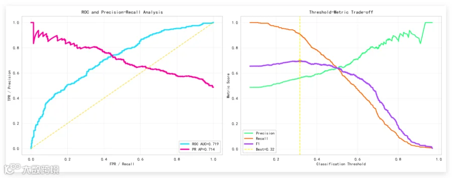
左图同时观察ROC和PR曲线。ROC越靠近左上角，说明模型区分能力越强；PR曲线更关注高风险客户有没有被准确找出来，适合类别不均衡场景。

右图展示分类阈值对业务结果的影响。提高阈值通常会提升Precision，但会降低Recall。黄色虚线对应F1最高的位置，不必固定使用0.5。

总结

数据类型转换的关键，是先理解字段含义，再决定如何解析。数字要去单位，日期要提取时间信息，类别要避免错误的大小关系，转换失败的数据则交给缺失值策略处理。