
哈喽,大家好~
今儿和大家详细的聊聊随机森林~
咱们先举一个例子:
当你在一个重要问题上要做判断,你不希望只听一个人的意见,因为那个人可能有偏见或偶然错误;更稳妥的方法是问一群人,每个人独立做判断,然后“投票取众”。随机森林就是机器学习里把这个想法量化的算法:它让很多“决策树”分别在稍有不同的数据/视角下做决定,最后把这些树的结果汇总(分类时投票,回归时取平均),通常得到比单棵树更稳健、更不容易过拟合的结果。
核心要点:
-
多个弱模型(决策树)合起来一个强模型。 -
通过引入随机性让个体之间“差异化”,避免大家都犯同样的错误。 -
可以量化“袋外误差”来估计泛化能力,不一定需要单独验证集。 -
输出还可以给出“特征重要性”,便于解释。
随机森林核心逻辑
随机森林通常基于 CART(Classification and Regression Trees)决策树。
核心包含两层“随机”:
-
数据随机:每棵树用原始训练集有放回采样得到的子样本训练,大约 63.2% 的样本会出现在某棵树的训练集中,剩下的样本称为该树的袋外(OOB)样本。 -
特征随机:每次节点分裂时,不在所有特征上寻找最优分割,而是在随机选择的 $m$ 个特征子集中寻找最优分割($m$ 通常为 $\sqrt{p}$ 或 $p/3$,$p$ 为特征总数),从而降低树之间的相关度。
决策树择分用的不纯度指标(以分类为例)常用 Gini:
$$Gini(S) = 1 - \sum_{k=1}^{K} p_k^2 $$其中 $p_k$ 是样本集 $S$ 中属于类别 $k$ 的比例。
某次按某特征与阈值划分为左右子集 $S_L, S_R$,不纯度减少量(基于 Gini)为:
$$\Delta Gini = Gini(S) - \frac{|S_L|}{|S|} Gini(S_L) - \frac{|S_R|}{|S|} Gini(S_R) $$树的训练过程就是在允许的特征子集上选择能最大化 $\Delta Gini$ 的分裂,递归建树直至满足停止条件(最大深度、最小样本数等)。
最终预测(分类)用多数投票:
$$\hat{y} = \text{mode}\{ T_1(x), T_2(x), ..., T_M(x)\} $$回归则取平均:
$$\hat{y} = \frac{1}{M}\sum_{m=1}^{M} T_m(x) $$袋外误差(OOB)可以直接用于估计泛化误差,因为对于某个样本,被某棵树训练所用的概率是 $\approx 1 - (1 - 1/n)^n \approx 1 - e^{-1} \approx 0.632$,所以有一部分树对该样本是“未见过”的,可以利用它们的投票来评估。
完整案例
我们试着用 PyTorch 从头实现一个简化版的随机森林分类器~
数据方面,我们使用 sklearn 的 make_moons 与 make_blobs 叠加产生复杂非线性、带噪声的数据(二维),便于可视化决策边界。
用 PyTorch 张量加速分割与统计(不是用 sklearn 的 RandomForest)。
为简捷,决策树取 CART 的基本策略,分裂阈值取特征值的中点(剪枝采用最大深度与最小样本数)。
import torch
import numpy as np
import matplotlib.pyplot as plt
from matplotlib.colors import ListedColormap
from sklearn.datasets import make_moons, make_blobs
from sklearn.metrics import confusion_matrix, roc_curve, auc
from sklearn.model_selection import train_test_split
import seaborn as sns
sns.set()

device = torch.device('cpu')

# 生成二维数据:moons + blobs 噪声叠加
np.random.seed(42)
X1, y1 = make_moons(n_samples=300, noise=0.15, random_state=0)
X2, y2 = make_blobs(n_samples=100, centers=[(2.5, 0.0)], cluster_std=0.25, random_state=1)
# 将 blob 的标签设为 1(与 moon 中的一类可能重合),为了制造复杂的重叠
X = np.vstack([X1, X2])
y = np.hstack([y1, np.ones(len(y2))])

# 打乱并切分训练/测试
X_train, X_test, y_train, y_test = train_test_split(X, y, test_size=0.25, random_state=42, stratify=y)
X_train = torch.tensor(X_train, dtype=torch.float32)
X_test  = torch.tensor(X_test,  dtype=torch.float32)
y_train = torch.tensor(y_train, dtype=torch.long)
y_test  = torch.tensor(y_test,  dtype=torch.long)
实现简化 CART 决策树:
class SimpleDecisionTree:
    def __init__(self, max_depth=6, min_samples_split=2, max_features=None):
        self.max_depth = max_depth
        self.min_samples_split = min_samples_split
        self.max_features = max_features  # number or None -> use all features
        self.tree = None

    def fit(self, X, y):
        X = X.clone()
        y = y.clone()
        n_features = X.shape[1]
        if self.max_features isNone:
            self.max_features = n_features
        self.n_classes = int(y.max().item() + 1)
        self.tree = self._build_tree(X, y, depth=0)

    def _gini(self, y):
        # y: 1D tensor of labels
        if y.numel() == 0:
            return0.0
        counts = torch.bincount(y, minlength=self.n_classes).float()
        p = counts / counts.sum()
        return1.0 - torch.sum(p * p)

    def _best_split(self, X, y):
        n_samples, n_features = X.shape
        best = {'feature': None, 'threshold': None, 'gain': 0.0, 'left_idx': None, 'right_idx': None}
        base_gini = self._gini(y)
        # 随机选特征子集
        feat_idx = np.random.choice(n_features, self.max_features, replace=False)
        for feat in feat_idx:
            vals = X[:, feat]
            # 候选阈值:按特征值的中点
            sorted_vals, idx = torch.sort(vals)
            # 仅在不同值之间考虑阈值
            thresholds = (sorted_vals[:-1] + sorted_vals[1:]) / 2.0
            if thresholds.numel() == 0:
                continue
            # Vectorized check: for each threshold compute gini
            for thr in thresholds:
                left_mask = vals <= thr
                right_mask = ~left_mask
                if left_mask.sum() < 1or right_mask.sum() < 1:
                    continue
                g_left = self._gini(y[left_mask])
                g_right = self._gini(y[right_mask])
                w_left = left_mask.sum().item() / n_samples
                w_right = right_mask.sum().item() / n_samples
                gain = base_gini - (w_left * g_left + w_right * g_right)
                if gain > best['gain']:
                    best.update({'feature': int(feat), 'threshold': float(thr.item()), 'gain': float(gain),
                                 'left_idx': left_mask, 'right_idx': right_mask})
        return best

    def _build_tree(self, X, y, depth):
        node = {}
        n_samples = y.numel()
        num_labels = torch.bincount(y, minlength=self.n_classes)
        pred_label = torch.argmax(num_labels).item()
        node['is_leaf'] = False
        node['prediction'] = int(pred_label)
        # stopping criteria
        if depth >= self.max_depth or n_samples < self.min_samples_split or (num_labels > 0).sum() == 1:
            node['is_leaf'] = True
            return node
        best = self._best_split(X, y)
        if best['feature'] isNoneor best['gain'] <= 1e-6:
            node['is_leaf'] = True
            return node
        # create children
        node['feature'] = best['feature']
        node['threshold'] = best['threshold']
        left_idx = best['left_idx']
        right_idx = best['right_idx']
        node['left'] = self._build_tree(X[left_idx], y[left_idx], depth + 1)
        node['right'] = self._build_tree(X[right_idx], y[right_idx], depth + 1)
        return node

    def _predict_one(self, x, node):
        if node['is_leaf']:
            return node['prediction']
        feat = node['feature']
        if x[feat] <= node['threshold']:
            return self._predict_one(x, node['left'])
        else:
            return self._predict_one(x, node['right'])

    def predict(self, X):
        X = X.clone()
        preds = []
        for i in range(X.shape[0]):
            preds.append(self._predict_one(X[i], self.tree))
        return torch.tensor(preds, dtype=torch.long)
实现随机森林:
class SimpleRandomForest:
    def __init__(self, n_estimators=20, max_depth=6, min_samples_split=2, max_features=None):
        self.n_estimators = n_estimators
        self.trees = []
        self.max_depth = max_depth
        self.min_samples_split = min_samples_split
        self.max_features = max_features
        self.oob_votes = None# for OOB evaluation
        self.feature_importances_ = None

    def fit(self, X, y):
        n_samples = X.shape[0]
        self.n_classes = int(y.max().item() + 1)
        self.trees = []
        # For OOB tracking: for each sample, accumulate votes from trees where sample was OOB
        oob_votes = [ [] for _ in range(n_samples) ]
        # feature importances: sum of gains per feature across trees
        feat_importances = torch.zeros(X.shape[1])
        for m in range(self.n_estimators):
            # bootstrap sample indices
            idxs = np.random.choice(n_samples, size=n_samples, replace=True)
            idxs = torch.tensor(idxs, dtype=torch.long)
            oob_mask = np.ones(n_samples, dtype=bool)
            oob_mask[idxs.numpy()] = False
            # train tree on bootstrap sample
            tree = SimpleDecisionTree(max_depth=self.max_depth, min_samples_split=self.min_samples_split,
                                      max_features=self.max_features)
            tree.fit(X[idxs], y[idxs])
            self.trees.append(tree)
            # accumulate OOB votes
            for i in range(n_samples):
                if oob_mask[i]:
                    pred = tree.predict(X[i:i+1])[0].item()
                    oob_votes[i].append(pred)
            # approximate feature importance by traversing tree and summing gains
            # NOTE: here our SimpleDecisionTree didn't store gain per split; for demo we approximate by counting usage
            # A better impl would return per-split gain. We'll approximate: count appearance of feature in tree nodes
            def traverse(node):
                if node.get('is_leaf', False):
                    return []
                feat = node.get('feature', None)
                res = [feat] if feat isnotNoneelse []
                res += traverse(node.get('left', {}))
                res += traverse(node.get('right', {}))
                return res
            used_feats = traverse(tree.tree)
            for f in used_feats:
                if f isnotNone:
                    feat_importances[f] += 1.0
        # compute OOB error
        oob_preds = []
        oob_true = []
        for i in range(n_samples):
            votes = oob_votes[i]
            if len(votes) == 0:
                continue
            counts = np.bincount(votes, minlength=self.n_classes)
            pred = np.argmax(counts)
            oob_preds.append(pred)
            oob_true.append(int(y[i].item()))
        if len(oob_preds) > 0:
            oob_preds = np.array(oob_preds)
            oob_true = np.array(oob_true)
            oob_err = 1.0 - np.mean(oob_preds == oob_true)
        else:
            oob_err = None
        self.oob_error_ = oob_err
        # normalize feature importances
        self.feature_importances_ = (feat_importances / feat_importances.sum()).numpy()
        return self

    def predict(self, X):
        # majority voting
        all_preds = []
        for tree in self.trees:
            all_preds.append(tree.predict(X).numpy())
        all_preds = np.stack(all_preds, axis=1)  # (n_samples, n_trees)
        final = []
        for row in all_preds:
            counts = np.bincount(row, minlength=self.n_classes)
            final.append(np.argmax(counts))
        return np.array(final)

    def predict_proba(self, X):
        # class probability by averaging one-hot votes
        all_preds = []
        for tree in self.trees:
            all_preds.append(tree.predict(X).numpy())
        all_preds = np.stack(all_preds, axis=1)  # (n_samples, n_trees)
        probs = []
        for row in all_preds:
            counts = np.bincount(row, minlength=self.n_classes).astype(float)
            probs.append(counts / counts.sum())
        return np.array(probs)
训练随机森林并画图(决策边界 / 数据分布 / 特征重要性 / OOB):
# 参数设置
n_estimators = 40
rf = SimpleRandomForest(n_estimators=n_estimators, max_depth=6, min_samples_split=2, max_features=1)  # max_features=1 -> random

rf.fit(X_train, y_train)
y_pred = rf.predict(X_test)
acc = (y_pred == y_test.numpy()).mean()
print(f"Test accuracy: {acc:.3f}, OOB error: {rf.oob_error_}")

# 1) 数据散点图(训练 / 测试)
plt.figure(figsize=(6,5))
cmap_bright = ListedColormap(['#FF3B30', '#34C759'])
plt.scatter(X_train[:,0], X_train[:,1], c=y_train, cmap=cmap_bright, edgecolor='k', alpha=0.7, label='train')
plt.scatter(X_test[:,0], X_test[:,1], c=y_test, cmap=cmap_bright, marker='^', edgecolor='k', alpha=1.0, label='test', s=80)
plt.title("Data distribution (bright colors)")
plt.legend()
plt.tight_layout()
plt.show()

# 2) 决策边界热力图
xx, yy = np.meshgrid(np.linspace(X[:,0].min()-0.5, X[:,0].max()+0.5, 300),
                     np.linspace(X[:,1].min()-0.8, X[:,1].max()+0.8, 300))
grid = np.c_[xx.ravel(), yy.ravel()]
grid_t = torch.tensor(grid, dtype=torch.float32)
Z = rf.predict(grid_t)
Z = Z.reshape(xx.shape)

plt.figure(figsize=(8,6))
cmap_bg = ListedColormap(['#FFEEEC', '#E8FFF1'])
plt.contourf(xx, yy, Z, alpha=0.6, cmap=ListedColormap(['#FFCCCB','#C8F7D6']))
plt.scatter(X[:,0], X[:,1], c=y, cmap=cmap_bright, edgecolor='k', s=30)
plt.title("Random Forest Decision Boundary (vivid palette)")
plt.tight_layout()
plt.show()

# 3) 特征重要性条形图
plt.figure(figsize=(6,4))
feats = np.arange(X.shape[1])
imp = rf.feature_importances_
colors = ['#FF9500', '#007AFF']
plt.bar(feats, imp, color=colors, edgecolor='k')
plt.xticks(feats, [f"f{int(i)}"for i in feats])
plt.title("Feature importances (approx)")
plt.ylabel("Relative importance")
plt.tight_layout()
plt.show()

# 4) OOB error 随树数变化(通过逐步训练近似)
# 为演示,我们按 1...n_estimators 分别训练多个 RF 并记录 OOB
oob_errs = []
for m in range(1, n_estimators+1):
    rf_m = SimpleRandomForest(n_estimators=m, max_depth=6, min_samples_split=2, max_features=1)
    rf_m.fit(X_train, y_train)
    oob_errs.append(rf_m.oob_error_)
plt.figure(figsize=(6,4))
plt.plot(range(1, n_estimators+1), oob_errs, '-o', color='#5856D6')
plt.xlabel("Number of trees")
plt.ylabel("OOB error")
plt.title("OOB error vs n_estimators")
plt.grid(alpha=0.3)
plt.tight_layout()
plt.show()

# 5) 混淆矩阵 & ROC(测试集)
cm = confusion_matrix(y_test.numpy(), y_pred)
plt.figure(figsize=(5,4))
sns.heatmap(cm, annot=True, fmt='d', cmap='YlGnBu', cbar=False)
plt.xlabel("Predicted")
plt.ylabel("True")
plt.title("Confusion Matrix (test)")
plt.tight_layout()
plt.show()

# ROC (二分类)
probs = rf.predict_proba(X_test)[:,1]
fpr, tpr, _ = roc_curve(y_test.numpy(), probs)
roc_auc = auc(fpr, tpr)
plt.figure(figsize=(5,4))
plt.plot(fpr, tpr, color='#FF2D55', lw=2, label=f'AUC = {roc_auc:.3f}')
plt.plot([0,1],[0,1], color='gray', linestyle='--')
plt.xlabel("FPR")
plt.ylabel("TPR")
plt.title("ROC Curve")
plt.legend(loc='lower right')
plt.tight_layout()
plt.show()
注意,我们在决策树实现中没有记录每次分裂的实际 gain 值(为保持代码简洁)。因此特征重要性这里采用“节点中被选用次数”作为近似量度(实际工程中应累计每次分裂带来的不纯度减少 $\Delta Gini$)。
训练时间与树的数量、数据量和 max_features 相关。我的实现是演示性质,适合教学与小数据测试;工业级随机森林建议使用 sklearn/LightGBM/XGBoost 等高效实现。
可视化分析
数据散点图:
直观观察数据在二维空间中的分布、标签类别及训练/测试划分。
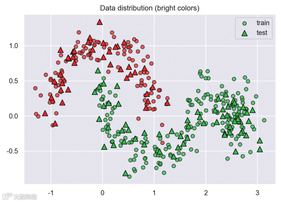
通过颜色和标记可以看到数据的非线性结构(moons)与局部簇(blobs),说明线性模型难以胜任。
随机森林决策边界:
可视化模型在整个输入空间的分类决策。
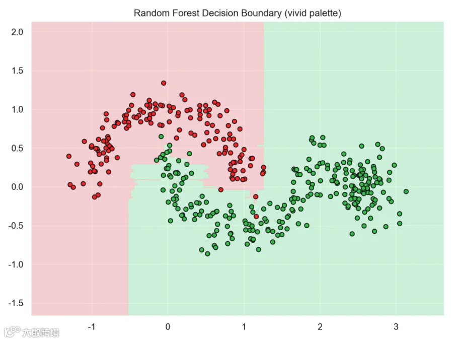
由于随机森林由多棵非线性树组成,边界通常呈阶梯状、分段包围类区域。能看到模型如何分离两个类、在重叠区域的模糊边界,以及是否产生过度分割(过拟合)。热力与点的叠加方便对比真实数据。
特征重要性:
评估不同特征对模型决策的贡献。
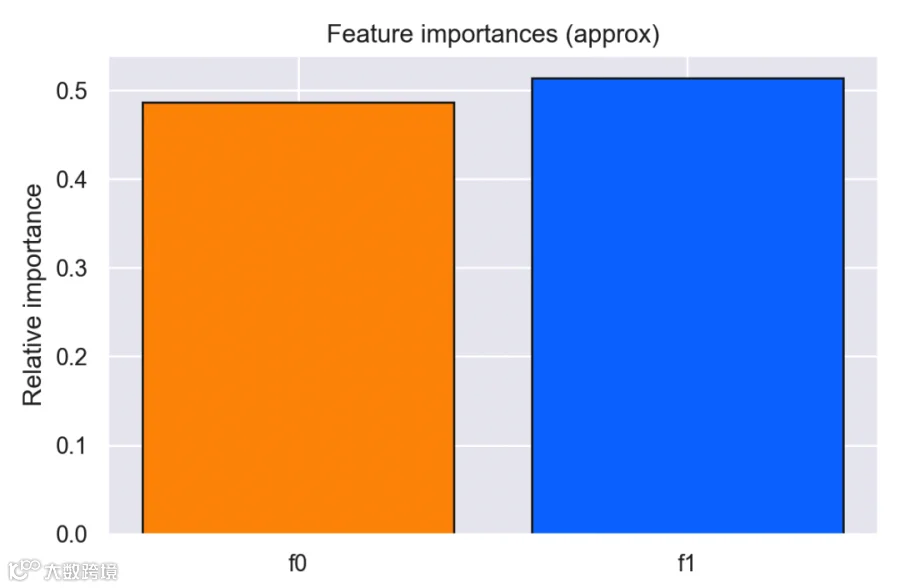
在合成数据中两维可能贡献不一样(例如 blob 的位置可能高度依赖 x 轴)。条形图能告诉我们哪一维更能区分类别,便于后续特征筛选或工程解释。
OOB 误差随树数变化:
展示树的数量如何影响泛化误差,是否持续下降或趋于稳定。
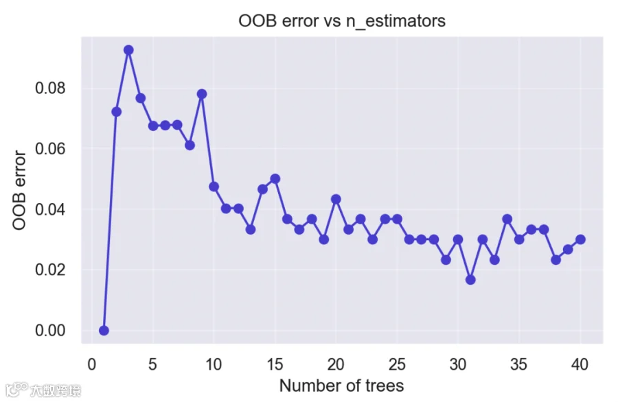
通常随着树数增加,OOB 误差会下降然后趋于平稳(方差减少,但偏差稳定)。这个图能帮助我们选择合适的树数(在耗时与效果间折中)。
混淆矩阵与 ROC 曲线:
定量评估预测性能和错误类型(误报/漏报)。
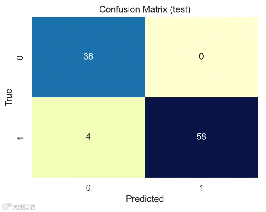
混淆矩阵告诉你模型在哪个类上更容易犯错;ROC/AUC 提供 threshold 不变情况下模型的整体判别能力(越接近 1 越好)。这些都是模型选择与迭代的重要指标。
总结
随机森林,通常效果稳健,抗噪声能力强,不容易过拟合,相较于单棵完整树。
可以处理高维数据、混合类型特征(数值、类别)。
自带特征重要性评估,便于解释。OOB 误差可用于模型监控而不需要独立验证集(节省数据)。
缺点也很明显,在高维稀疏问题上(如文本)可能不如线性模型或基于树的梯度提升在速度与效果上优秀。
另外,模型体积较大,可解释性不如单棵树。
最后
最近准备了16大块的内容,124个算法问题的总结,完整的机器学习小册,免费领取~