从零构建一个 200M 参数的时间序列 LLM

用于 zero-shot 预测的 decoder-only patched transformer

构建一个能处理从未见过的序列的单一预测模型，而不是为每个数据集重新训练一个新模型，仍然是一个难题。这个领域正在收敛到一个答案：把预测当作语言建模来做。Decoder-only transformers，也就是现代语言模型背后的架构，已经成为预测领域最强的方法之一，而且 Google 最近发布的基于 decoder 的模型达到了传统方法无法匹敌的准确率。因此我决定从头解决这个问题：从零构建模型和完整训练 pipeline，并把它扩展到2 亿参数。

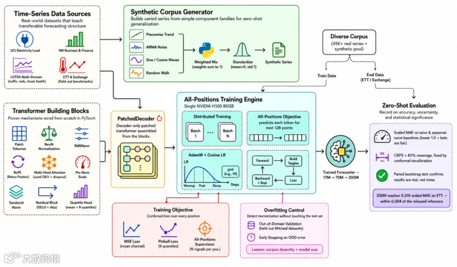
我们要构建的模型是一个 patched decoder，它由六个部分组成：

• Patch tokenizer：把每个包含 32 个数值的窗口转换成一个 token。

• RevIN normalization：重新缩放每个窗口，使其单位和量级不再重要。

• Decoder stack：transformer layers，其中每个 token 只能回看更早的 token。

• Quantile head：输出不确定性区间，而不是单个数值。

• All-positions training：每个 token 都预测它后面的那一段。

• Autoregressive forecast：向前滚动，把每次预测反馈回去，从而把预测延长到所需长度。

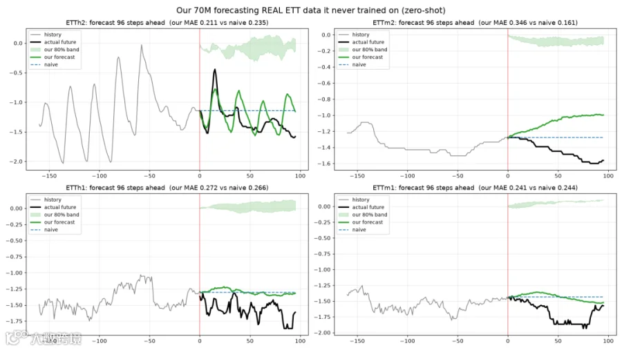
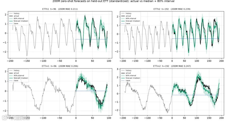
我想做的是一个模型：给它一个从未见过的序列，它能返回一个预测，并带有合理的不确定性区间。最终效果如下。在单块 GPU 上连续训练200M 模型约9 小时后，绿色预测线能跟踪它从未见过的序列，黑色是真实值。

在这篇博客中，我们将从零构建这个 decoder-only forecaster，包括模型和完整训练 pipeline，并从一个很小的17M 版本一路扩展到上面的200M 版本。我们会逐步推进，在每个规模上遇到问题、修复问题。

我训练好的模型权重在这里：

https://huggingface.co/FareedKhan/timesfm-from-scratch-70m

所有代码都在我的 GitHub repository 中：

https://github.com/FareedKhan-dev/timesfm-from-scratch

目录

• 目标：预测模型从未见过的序列

• 我们要构建什么，以及如何衡量它

• 代码库地图

• Setup 和 imports

• Synthetic data generator

• Patches as tokens，以及 RevIN normalization

• Transformer block，逐个机制构建∘ ResidualBlock 和 RMSNorm∘ RoPE 和逐维 scale∘ Multi-head attention：fused QKV、qk-norm 和 unit scale∘ Sandwich norm 和双矩阵 feed-forward

• 组装完整模型和 forward pass∘ 从训练输出到 autoregressive forecast

• 目标函数：预测接下来的每个 128 个点

• 训练循环：optimizer 和 schedule

• 在 synthetic data 上训练 17M 模型

• 扩展到 70M，以及“数据胜过规模”的教训

• 过拟合问题

• 修复：corpus 多样性

• 一个 bug：模型在起点处最弱

• 评估 harness

• Random-walk 数据，以及一个部分修复

• 校准不确定性：conformal recalibration

• 扩展到 200M 模型

• 局限性和下一步我会构建什么

• 构建过程教会我的事

目标：预测模型从未见过的序列

先把目标说具体。我们想要一个模型，它接收某个序列的历史值，比如小时级电力负荷、日级网站流量或货币汇率，然后预测接下来的一段，即使它之前从未见过这个具体序列。

Zero-shot forecasting 很难，因为模型可以完美拟合一个数据集，却在新数据集上毫无用处；它学到的是那个数据集的怪癖，而不是时间序列的一般语法。目标是学习可迁移的结构，也就是跨成千上万个来源都会出现的 seasonality、trend 和 noise，而不是偷看我们要测试的序列。

这篇博客中的几乎每个设计决策，都是为了把模型推向这种可迁移结构，并远离记忆。

我们要构建什么，以及如何衡量它

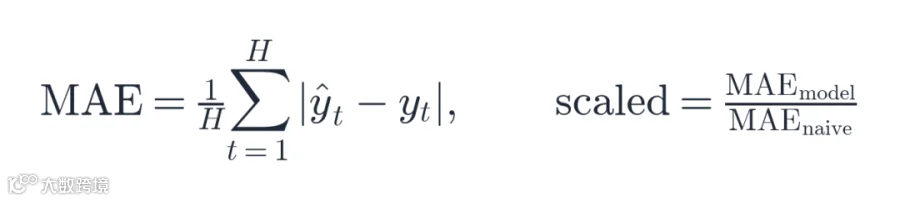
在构建任何东西之前，我需要知道如何判断它是否有效。指标是scaled MAE，即我们预测的 mean absolute error 除以一个 naive baseline 的 mean absolute error；这个 baseline 只是把最后一个值向前重复。低于1.0 就说明我们击败了 baseline，高于1.0 则说明还不如不做任何聪明处理。

benchmark 是 held-outETT dataset（electricity transformer temperature），模型从不在它上面训练。作为尺度参考，一个强大的公开200M forecasting model 在这里大约得0.215，这就是我们最终模型的目标。

模型有三种尺寸，贯穿全文使用：tiny、small 和base，只由 model dimension 和 layer 数决定。sanity script 会构建三者并打印参数量。

#### OUTPUT #### === param counts === tiny 17.65M dim=512 layers=10 heads=16 head_dim=32 outputs=10 small 67.80M dim=1024 layers=10 heads=16 head_dim=64 outputs=10 base 203.44M dim=1280 layers=20 heads=16 head_dim=80 outputs=10

这就是我们的三阶梯：用17.65M 快速 debug，用67.80M 学习什么真正驱动预测质量，用203.44M 作为最终目标模型，它匹配已发布参考模型的 backbone size。最后一列outputs=10 是均值加九个 quantiles，等到 loss 部分我们会看到原因。

代码库地图

这样的项目有很多移动部件，但依赖流很简单。Config 定义尺寸，layers 和 normalization 喂给 model，model 和 loss 喂给 trainer，data loaders 也喂给 trainer，而 evaluation scripts 产生本文中的每个数字和图。

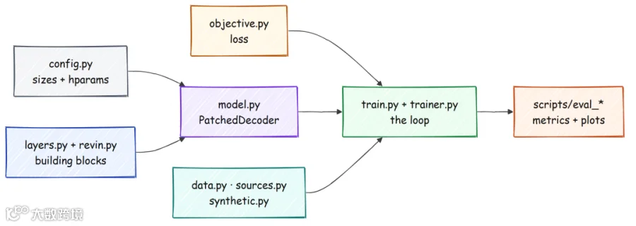
下面是源码布局，方便你按文件跟读。

tsfm-scratch/ src/tsfm/ config.py # model + training config, the three size presets revin.py # reversible instance normalization (per-series scaling) layers.py # ResidualBlock, RMSNorm, RoPE, attention, transformer block model.py # PatchedDecoder: the full forward pass + autoregressive forecast objective.py # the all-positions loss (MSE + pinball quantile loss) trainer.py # optimizer, LR schedule, one training step, OOD validation synthetic.py # the synthetic time-series generator data.py # windowing + the random-prefix masking trick sources.py # real-data loaders (electricity, M4, LOTSA) scripts/ sanity.py # param counts + one forward/backward pass overfit_one_batch.py # the correctness gate train.py # the training entrypoint eval_core.py # the shared evaluation protocol + metrics eval_multidomain.py # the multi-domain zero-shot test grid

我们会大致自上而下构建它。先是模型要学习的数据，然后是模型本身，再是 loss 和训练循环，最后沿着三个尺寸逐步爬升。

先从环境开始。

Setup 和 imports

依赖列表刻意保持很小。核心 package 只需要 NumPy，PyTorch 是用于实际训练的 optional extra。

[project] name = "tsfm" version = "0.1.0" description = "From-scratch decoder-only time-series foundation model + training pipeline" requires-python = ">=3.10" dependencies = ["numpy>=1.26"] [project.optional-dependencies] torch = ["torch>=2.2"] dev = ["pytest>=8"]

我用uv 安装，这能保持环境可复现；所有实验都在本地一台带单块NVIDIA H100 80GB 的 GPU 机器上运行。

uv venv uv pip install -e ".[torch,dev]"

第一段代码是 configuration object。模型需要的每个 hyperparameter 都放在一个 dataclass 中，两个 computed properties 避免我们到处重复算术。

@dataclass class ModelConfig: model_dim: int = 1280 num_layers: int = 20 num_heads: int = 16 patch_len: int = 32 horizon_len: int = 128 quantiles: Tuple[float, ...] = (0.1, 0.2, 0.3, 0.4, 0.5, 0.6, 0.7, 0.8, 0.9) dropout: float = 0.0 rope_max_period: float = 10000.0 rms_eps: float = 1e-6 @property def head_dim(self) -> int: assert self.model_dim % self.num_heads == 0 return self.model_dim // self.num_heads @property def num_outputs(self) -> int: return 1 + len(self.quantiles) # mean (point) + quantiles

其中几项值得停一下，因为它们定义了后续所有形状。patch_len 为32，表示一个 token 由多少个 raw points 组成。

horizon_len 为128，表示模型一次预测多远。quantiles tuple 有九个条目，所以num_outputs 是10：一个 channel 给 mean，另外九个给 quantiles。

这个小细节就是 sanity print 中outputs=10 的原因，也正是它让模型能表达不确定性，而不是只给一个猜测值。

Synthetic data generator

第一个问题来了。要训练一个能跨多类序列泛化的模型，我们需要大量多样化序列。

我没有一个现成的巨大标注 corpus，所以自己“种”一个。Synthetic generator 把一个序列构造成几类简单 component 的加权和：trend、ARMA noise、sine 和 cosine waves，并加入一部分纯 random walk。

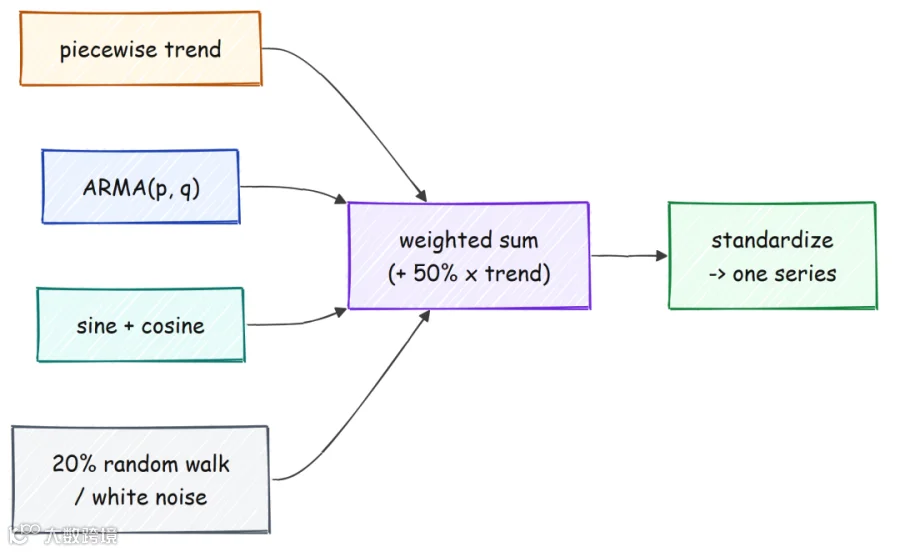
我们一次构建一个 component family。最有意思的是 ARMA，即 autoregressive moving-average process，因为我在这里遇到了第一个 bug。

要生成 ARMA series，我们需要能产生稳定过程的 coefficients。如果随便选，过程会爆炸到无穷大，导致 NaNs。

稳定性的条件是 characteristic polynomial 的所有 roots 都严格位于 unit circle 内部。

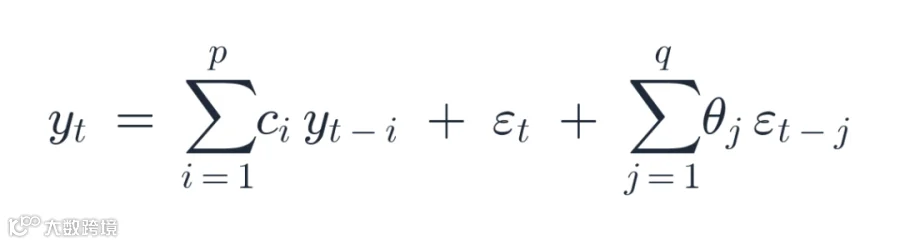
def _reject_sample_roots(rng, order, max_attempts=200): """Sample stationary AR (or invertible MA) coefficients. For y_t = c1 y_{t-1} + ... + cp y_{t-p} + e_t the characteristic polynomial is z^p - c1 z^{p-1} - ... - cp; the process is stationary iff ALL roots lie INSIDE the unit circle. """ for _ in range(max_attempts): c = rng.normal(0, 0.4, size=order) roots = np.roots(np.concatenate([[1.0], -c])) # char poly z^p - c1 z^{p-1} - ... if np.all(np.abs(roots) < 0.99): return c return np.array([0.5] + [0.0] * (order - 1)) # AR(1), c=0.5 -> stationary fallback

这个函数通过 rejection sampling 采样 stable coefficients。我的第一个版本把测试写反了：它保留会爆炸的 coefficients，却拒绝好的 coefficients。于是每隔几个 batch 就会有序列爆到 infinity，污染 loss。

修复就是那一行：检查 roots 在圆内。

ARMA recurrence 本身是标准形式：下一个值是过去值的加权和，加上过去噪声项的加权和。

wave components 更简单。随机选 period、phase 和 amplitude，然后在整个序列长度上计算 sine 或 cosine。

def generate_wave(length, rng, fn): period = float(rng.integers(4, max(5, length // 2 + 1))) phase = float(rng.uniform(0, 2 * np.pi)) amp = float(np.clip(rng.normal(1.0, 0.5), 0.1, 3.0)) t = np.arange(length, dtype=np.float32) return (amp * fn(2 * np.pi * t / period + phase)).astype(np.float32)

trend component 是一条 piecewise-linear walk。我们选几个 segments，给每段一个随机 slope，并在 breakpoints 处拼接保持连续，从而得到中途会弯折的趋势，而不是永远一条直线。

def generate_piecewise_trend(length, rng): k = int(rng.integers(2, 9)) # 2..8 segments bp = np.sort(rng.choice(np.arange(1, length), size=k - 1, replace=False)) if k > 1 else np.array([], int) breaks = np.concatenate([[0], bp, [length]]).astype(int) slopes = rng.normal(0, 0.5, size=k) trend = np.zeros(length, np.float32) intercept = 0.0 for i in range(k): t0, t1 = breaks[i], breaks[i + 1] t = np.arange(t0, t1, dtype=np.float32) trend[t0:t1] = intercept + slopes[i] * (t - t0) if t1 > t0: intercept = float(trend[t1 - 1]) # keep the line continuous at each break return trend

ARMA component 需要刚才采样的 stable coefficients。它在 burn-in period 加上目标长度上向前运行 recurrence，然后丢掉 burn-in，使过程在保留之前已经进入自然行为状态。

def generate_arma(length, rng, max_attempts=100): p = int(rng.integers(1, 9)) q = int(rng.integers(1, 9)) ar = _reject_sample_roots(rng, p, max_attempts) # stationary AR coefficients ma = _reject_sample_roots(rng, q, max_attempts) # invertible MA coefficients burn = max(p, q) * 10 # let the process forget its zero start n = burn + length eps = rng.normal(0, 1.0, size=n) y = np.zeros(n, np.float32) for t in range(n): pp = min(p, t); qq = min(q, t) ar_part = float(np.dot(ar[:pp], y[t - pp:t][::-1])) if pp else 0.0 ma_part = float(np.dot(ma[:qq], eps[t - qq:t][::-1])) if qq else 0.0 y[t] = ar_part + eps[t] + ma_part return y[burn:].astype(np.float32)

我们刚构建了两个最难的 component family。trend generator 产生连续弯折线，ARMA generator 产生相关噪声，并带有我们保证的稳定性。

burn-in 设为 model order 的十倍，这是重要细节：它让过程忘记从零开始这件事，在我们切出保留部分之前达到自然方差。

现在组装完整序列。我们随机打开或关闭每个 component family，用和为一的随机权重混合 active components，以 additive 或 multiplicative 方式应用 trend，并标准化结果。

def generate_series(length, rng, rw_prob=0.2): if rng.random() < rw_prob: # ~20% structureless RW/white-noise y = generate_random_walk(length, rng) else: on = {k: bool(rng.random() < 0.5) for k in ("trend", "arma", "sine", "cosine")} if not any(on.values()): on[("trend", "arma", "sine", "cosine")[int(rng.integers(0, 4))]] = True comp = {} if on["trend"]: comp["trend"] = generate_piecewise_trend(length, rng) if on["arma"]: comp["arma"] = generate_arma(length, rng) if on["sine"]: comp["sine"] = generate_wave(length, rng, np.sin) if on["cosine"]: comp["cosine"] = generate_wave(length, rng, np.cos) names = list(comp) w = rng.uniform(0, 1, size=len(names)) w = w / w.sum() y_add = np.zeros(length, np.float32) for name, wi in zip(names, w): if name != "trend": y_add += wi * comp[name] if "trend" in comp: # trend can be additive or multiplicative tr = comp["trend"] wt = float(w[names.index("trend")]) denom = 1.0 + float(np.std(np.abs(tr))) if rng.random() < 0.5: y = (1.0 + wt * (tr / denom)) * y_add else: y = wt * tr + y_add else: y = y_add if rng.random() < 0.1: y = y + rng.normal(0, 0.1, size=length) y = np.nan_to_num(y, nan=0.0, posinf=0.0, neginf=0.0) # never emit nan/inf y = np.clip(y, -1e4, 1e4) s = float(y.std()) if s > 1e-6: y = (y - float(y.mean())) / s # standardize to ~unit scale return y.astype(np.float32)

这个generate_series 函数是 data pipeline 的核心，所以回顾一下它做了什么。它为每个 component 掷骰子，用 normalized weights 混合 active components，偶尔把 trend 作为乘法项而不是加法项，并总是在最后清理 NaN 或 infinity，把序列标准化到近似 unit scale。

顶部的rw_prob=0.2 分支，也就是 random walk，是我们后面为某个具体失败加入的修复，先记住它。

生成一个小 batch 看看统计量。

from tsfm.synthetic import make_batch batch = make_batch(4, 1024, seed=1) print("shape:", batch.shape) print("per-series mean:", batch.mean(axis=1).round(3)) print("per-series std :", batch.std(axis=1).round(3))

#### OUTPUT #### shape: (4, 1024) per-series mean: [ 0. -0. -0. 0. ] per-series std : [1. 1. 1. 1.]

每个序列的均值为零、标准差为一，这正是我们要求的。这是刻意设计的第一层 normalization，模型还有第二层 normalization（接下来构建），用于处理每个 context window 的 scale。

标准化 raw series 能让 synthetic magnitudes 保持合理，避免训练发散，并在模型看到任何数据之前让每个序列处在可比较的尺度上。

Patches as tokens，以及 RevIN normalization

我们有了序列。现在要把它们变成 transformer 能读取的形式。

这里发生两件事。我们把序列切成固定长度 patches，并对每个 window 进行 normalization，让模型关注形状而不是单位。

先看 patching 和 masking。序列被 reshape 成 N 个长度为 p 的 patches，所以一个长度 512、patch length 为 32 的 context 会变成 16 个 patches。

下面这个函数把 series list window 成一个 batch，并加入 masking。里面有一个聪明技巧：random-prefix mask。

def batch_from_series(series_list, context_len, patch_len, rng, device="cpu"): """Window each series to context_len, left-pad short ones, add the random-prefix mask.""" B = len(series_list) X = np.zeros((B, context_len), np.float32) P = np.zeros((B, context_len), np.float32) for i, s in enumerate(series_list): s = np.asarray(s, np.float32) if len(s) >= context_len: st = int(rng.integers(0, len(s) - context_len + 1)) X[i] = s[st:st + context_len] else: X[i, context_len - len(s):] = s # left-pad short series P[i, :context_len - len(s)] = 1.0 # mark the padding r = int(rng.integers(0, patch_len)) # random-prefix mask P[i, :r] = 1.0 return (torch.from_numpy(X).to(device), torch.from_numpy(P).to(device))

我们刚构建了 windower。对每条序列，如果足够长就取一个随机 window；否则 left-pad，并标记 padding。

然后它在序列开头 mask 掉随机数量的点，范围是零到一个完整 patch。为什么要 mask 一个 random prefix？

因为 inference 时模型会看到各种可能长度的 context，而不只是整齐地被 patch size 整除的长度。训练时 mask 一个 random prefix，模型就会学会处理各种 alignment，因此面对不能整除的 context 时不会意外。

现在是第二层 normalization，也是让模型 scale-blind 的那一层。它叫RevIN，即 reversible instance normalization。

思路是：用 context 第一个 patch 的 mean 和 standard deviation 标准化整个 context，在 normalized space 中运行模型，然后在 output 上反向 normalization。数值上千的电力负荷和接近一的汇率都会变成同一种标准化形状，所以模型只需要学习形状。

这里有个陷阱，让我浪费了一次训练。如果第一个 patch 恰好几乎是平的，它的 standard deviation 接近零，除以它会把 normalized values 送到 infinity。

修复方法是把 standard deviation floor 到整个 context standard deviation 的一个比例，并把 normalized values clamp 到安全范围。

def first_patch_stats(xp, pp, min_valid: int = 3, eps: float = 1e-6, ctx_floor: float = 0.3): """xp, pp: [B, N, p]; pp 1=pad/missing. Returns mu, sigma: [B]. Centers on the first valid patch (>=min_valid points), but FLOORS sigma at ctx_floor * the whole-context std so a near-flat first patch can't blow up the normalized scale (stability). """ B, N, p = xp.shape valid = 1.0 - pp # 1 = usable point counts = valid.sum(-1) # [B, N] has = counts >= min_valid # [B, N] idx = torch.argmax(has.to(torch.int64), dim=1) # first patch with enough real points none = ~has.any(dim=1) idx = torch.where(none, torch.full_like(idx, N - 1), idx) rows = torch.arange(B, device=xp.device) arr = xp[rows, idx] # [B, p] m = valid[rows, idx] n = m.sum(-1).clamp(min=1.0) mu = (arr * m).sum(-1) / n # mean of the first valid patch var = (((arr - mu[:, None]) * m) ** 2).sum(-1) / n sigma = var.clamp(min=0.0).sqrt() # whole-context std (over all valid points) as a stability floor cnt = valid.sum(dim=(1, 2)).clamp(min=1.0) gmu = (xp * valid).sum(dim=(1, 2)) / cnt gvar = (((xp - gmu[:, None, None]) * valid) ** 2).sum(dim=(1, 2)) / cnt ctx_std = gvar.clamp(min=0.0).sqrt() sigma = torch.maximum(sigma, ctx_floor * ctx_std) # the floor: at least 30% of the context std sigma = torch.where(sigma < eps, torch.ones_like(sigma), sigma) return mu, sigma

仔细读一下，因为 floor 是这里最重要的部分。

• mu 是第一个至少有三个真实点的 patch 的 mean。

• sigma 是同一个 patch 的 standard deviation。

• The floor 把 sigma 提升到至少为 whole-context standard deviation 的 30%，所以平坦的第一个 patch 永远不会产生很小的除数。

• The clamp（在模型中应用，到正负 20）捕捉仍然漏过的异常情况。

模型 forecast 时会反向操作：乘以 sigma，再加上 mu，把预测放回原始尺度。

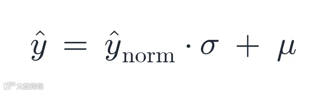
看一下 RevIN 在一个 batch 上的效果。

xp = x.view(B, -1, cfg.patch_len) pp = pad.view(B, -1, cfg.patch_len) mu, sigma = first_patch_stats(xp, pp) xn = ((xp - mu[:, None, None]) / sigma[:, None, None]).clamp(-20.0, 20.0) print("mu :", mu.numpy().round(3)) print("sigma:", sigma.numpy().round(3)) print("normalized range:", float(xn.min()), "to", float(xn.max()))

#### OUTPUT #### mu : [ 0.214 -1.880 0.061 0.945] sigma: [0.973 1.041 0.887 1.006] normalized range: -4.118 to 5.272

每个序列都有自己的 mu 和 sigma，normalization 后的值落在整洁范围内，远在正负 20 的 clamp 以内。这里 clamp 没有触发，这是我们希望的；它是 pathological cases 的护栏，而不是正常数据应该经常撞到的东西。

完成 patching 和 RevIN 后，模型终于有了能读取的 tokens。

Transformer block，逐个机制构建

现在构建 transformer 本身。我会把它拆成命名部件逐个组装，并解释每个部件为什么存在。

这里的每个机制都来自已知有效的设计，所以我们不是在猜，而是在按正确顺序把经过验证的部分接起来。

ResidualBlock 和 RMSNorm

第一个 building block 是一个带 skip connection 的小型 two-layer network，既用于输入 tokenizer，也用于输出 prediction head。它让输入经过一个带 SiLU activation 的 hidden layer，再经过 output layer，然后加上输入的 linear projection。

class ResidualBlock(nn.Module): def __init__(self, in_dim: int, hidden_dim: int, out_dim: int, bias: bool = False): super().__init__() self.hidden_layer = nn.Linear(in_dim, hidden_dim, bias=bias) self.output_layer = nn.Linear(hidden_dim, out_dim, bias=bias) self.residual_layer = nn.Linear(in_dim, out_dim, bias=bias) self.act = nn.SiLU() def forward(self, x): return self.output_layer(self.act(self.hidden_layer(x))) + self.residual_layer(x)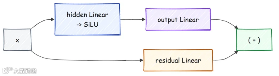

第二个 building block 是 transformer 内部使用的 normalization：RMSNorm。它用 root-mean-square 重新缩放向量，然后应用一个 learned per-dimension gain。

gain 初始化为零，所以(1 + scale) 一开始为一，layer 初始近似 identity，这能稳定早期训练。

class RMSNorm(nn.Module): def __init__(self, dim: int, eps: float = 1e-6): super().__init__() self.eps = eps self.scale = nn.Parameter(torch.zeros(dim)) # zero-init -> (1+scale) ~ identity at start def forward(self, x): dt = x.dtype xf = x.float() xf = xf * torch.rsqrt(xf.pow(2).mean(-1, keepdim=True) + self.eps) return (xf * (1.0 + self.scale.float())).to(dt)

我们刚构建了两个主力部件。ResidualBlock 是带内置 shortcut 的灵活 learned transformation，RMSNorm 是便宜、稳定且初始为 identity 的 normalization。

从这里开始它们会到处使用。

RoPE 和逐维 scale

Transformer 需要知道 token 的顺序。我们用rotary position embedding，也就是 RoPE，来编码位置；它根据位置把每个 query 和 key vector 旋转一个角度。

角度随 position 增大，并随 dimension index 缩小，所以不同维度以不同速率旋转。

class RotaryEmbedding(nn.Module): def __init__(self, head_dim: int, max_period: float = 10000.0): super().__init__() self.head_dim = head_dim self.max_period = max_period def cos_sin(self, positions, dtype): # positions: [N] -> cos/sin: [N, head_dim/2] half = self.head_dim // 2 device = positions.device freq = self.max_period ** (2.0 * torch.arange(half, device=device).float() / self.head_dim) ang = positions.float()[:, None] / freq[None, :] return torch.cos(ang).to(dtype), torch.sin(ang).to(dtype) @staticmethod def apply(x, cos, sin): # x: [B, H, N, D]; cos/sin: [N, D/2] first, second = x.chunk(2, dim=-1) cos = cos[None, None] sin = sin[None, None] return torch.cat([first * cos - second * sin, second * cos + first * sin], dim=-1)

attention 还配有一个小部件：query 上的 learnedper-dimension scale。我们不用常见的固定 one-over-square-root-of-d temperature，而是让模型通过 softplus 学习一个 per-dimension gain，并保持它为正。

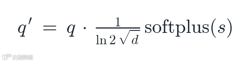
class PerDimScale(nn.Module): def __init__(self, dim: int): super().__init__() self.scale = nn.Parameter(torch.zeros(dim)) self.r = 1.442695041 / math.sqrt(dim) # 1/ln(2) / sqrt(d) def forward(self, x): return x * (self.r * F.softplus(self.scale))

Multi-head attention：fused QKV、qk-norm 和 unit scale

现在是 attention 本身。这里有几个有意为之的选择。

query、key 和 value projections 被fused 到一个 linear layer 中以提升速度。queries 和 keys 在 rotation 前分别经过自己的 RMSNorm，从而控制 magnitudes。

RoPE 应用于二者，per-dimension scale 应用于 query，实际 attention 使用1.0 的 scale，因为 temperature 已经由 per-dimension scale 处理。

class MultiHeadAttention(nn.Module): def __init__(self, cfg): super().__init__() d, self.h, self.hd = cfg.model_dim, cfg.num_heads, cfg.head_dim self.qkv = nn.Linear(d, 3 * d, bias=False) # fused Q, K, V in one matmul self.out = nn.Linear(d, d, bias=False) self.q_norm = RMSNorm(self.hd, cfg.rms_eps) # qk-norm on the query self.k_norm = RMSNorm(self.hd, cfg.rms_eps) # qk-norm on the key self.rope = RotaryEmbedding(self.hd, cfg.rope_max_period) self.per_dim = PerDimScale(self.hd) def forward(self, x, attn_mask, cos, sin): B, N, D = x.shape q, k, v = self.qkv(x).chunk(3, dim=-1) # split the fused projection q = self.q_norm(q.view(B, N, self.h, self.hd)) k = self.k_norm(k.view(B, N, self.h, self.hd)) v = v.view(B, N, self.h, self.hd) q, k, v = (t.transpose(1, 2) for t in (q, k, v)) # [B, H, N, hd] q = self.rope.apply(q, cos, sin) # rotate the query k = self.rope.apply(k, cos, sin) # rotate the key q = self.per_dim(q) # learned temperature on q o = F.scaled_dot_product_attention(q, k, v, attn_mask=attn_mask, scale=1.0) o = o.transpose(1, 2).reshape(B, N, D) return self.out(o)

我们刚构建了 attention。fused QKV 只需一次 matmul 而不是三次，queries 和 keys 在旋转前被 normalized，softmax temperature 是 learned 而不是 fixed。

attn_mask 参数用于保持模型 causal，我们马上会在模型本身中构建这个 mask。

Sandwich norm 和双矩阵 feed-forward

最后一个部件是包裹 attention 和 feed-forward network 的 block。这里的 norm placement 是sandwich：每个 sublayer 前后都有 normalization，而不只是前面有。

feed-forward 是两矩阵结构，中间是 SiLU，比 gated variants 更简单，并且正是我们所遵循的设计使用的形式。

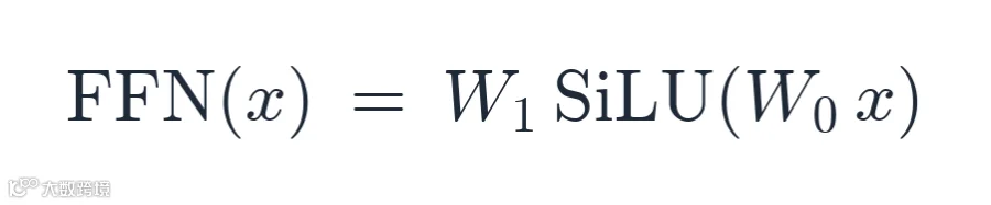
class TransformerBlock(nn.Module): def __init__(self, cfg): super().__init__() d = cfg.model_dim self.pre_attn_ln = RMSNorm(d, cfg.rms_eps) self.post_attn_ln = RMSNorm(d, cfg.rms_eps) self.attn = MultiHeadAttention(cfg) self.pre_ff_ln = RMSNorm(d, cfg.rms_eps) self.post_ff_ln = RMSNorm(d, cfg.rms_eps) self.ff0 = nn.Linear(d, d, bias=False) self.ff1 = nn.Linear(d, d, bias=False) self.act = nn.SiLU() self.drop = nn.Dropout(cfg.dropout) def forward(self, x, attn_mask, cos, sin): a = self.attn(self.pre_attn_ln(x), attn_mask, cos, sin) x = x + self.post_attn_ln(self.drop(a)) # sandwich: norm before AND after f = self.ff1(self.act(self.ff0(self.pre_ff_ln(x)))) x = x + self.post_ff_ln(self.drop(f)) return x

我们刚构建了一个完整 transformer block。输入先 normalization、attention、再 normalization 并加回，然后同样的 sandwich pattern 包裹 feed-forward。

堆叠多个这样的 block，就得到模型主体。

组装完整模型和 forward pass

所有部件都有了。现在把它们接进PatchedDecoder。

tokenizer 是一个ResidualBlock，接收 patch 及其 mask，产生 model-dimension embedding。主体是 transformer blocks 的 stack。

head 是另一个ResidualBlock，把最终 embedding 映射到完整 forecast，即每个 horizon step 乘以每个 output channel。

class PatchedDecoder(nn.Module): def __init__(self, cfg): super().__init__() self.cfg = cfg p = cfg.patch_len self.tokenizer = ResidualBlock(2 * p, cfg.model_dim, cfg.model_dim, bias=True) self.layers = nn.ModuleList([TransformerBlock(cfg) for _ in range(cfg.num_layers)]) self.rope = RotaryEmbedding(cfg.head_dim, cfg.rope_max_period) self.head = ResidualBlock(cfg.model_dim, cfg.model_dim, cfg.horizon_len * cfg.num_outputs, bias=False)

注意 tokenizer 接收2 * p 个输入，而不是p。因为我们把 normalized patch values 和 patch mask 拼接后喂给它，所以模型总知道哪些点是真实的，哪些是 padding。

head 输出horizon_len * num_outputs 个数，我们把它 reshape 成 horizon-by-channels grid。

现在是 forward pass。patching、RevIN、tokenizer、RoPE、mask 和 transformer stack 都在这里汇合。

def encode(self, x, padding): """Returns normalized per-position outputs [B, N, horizon, Q] + (mu, sigma).""" cfg = self.cfg p = cfg.patch_len B, L = x.shape assert L % p == 0, "context length must be a multiple of patch_len" N = L // p xp = x.view(B, N, p) pp = padding.view(B, N, p) mu, sigma = first_patch_stats(xp, pp) # RevIN stats xn = ((xp - mu[:, None, None]) / sigma[:, None, None]).clamp(-20.0, 20.0) xn = xn * (1.0 - pp) # zero out masked points tok_in = torch.cat([xn, pp], dim=-1) # [B, N, 2p]: values + mask h = self.tokenizer(tok_in) # [B, N, D] pos = torch.arange(N, device=x.device) cos, sin = self.rope.cos_sin(pos, h.dtype) patch_valid = pp.min(dim=-1).values < 0.5 # [B, N] True if any valid point mask = self._attn_mask(patch_valid) for blk in self.layers: h = blk(h, mask, cos, sin) out = self.head(h).view(B, N, cfg.horizon_len, cfg.num_outputs) return out, (mu, sigma)

把整个 forward pass 的 shapes 从头到尾追踪一次会很有帮助：

1. raw context 以[B, L] 形式到达，即 B 条序列，每条 L 个点。

2. reshape 成[B, N, p]，即 N 个 patches，每个 p 个点。

3. RevIN 为每条序列计算 mean 和 standard deviation 并 normalize，使每条序列落入相同的整洁范围。

4. 我们把 normalized values 和 padding mask 拼接，因此每个 token 宽度为2p，并携带自己的“哪些点是真实的”标记。

5. tokenizer 把每个 token 映射到 model dimension，得到[B, N, D]。

6. transformer stack 运行 L 个 blocks，形状保持[B, N, D]，但每个 patch 都被之前 patches 的信息丰富起来。

7. head 把每个 patch 扩展为[B, N, horizon, 10]，即一个 128-step forecast，每步十个 channels。

每一步都保持 batch 和 patch dimensions，这正是一个 forward pass 能同时在每个位置产生预测的原因，也是 decoder-only objective 的效率所在。

output shape 表示模型产生什么：对序列中的每个位置，模型预测接下来的 128 步，并为每一步产生 10 个 channels：mean 加九个 quantiles。

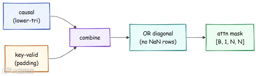
def _attn_mask(self, patch_valid): # patch_valid: [B, N] bool. Returns [B, 1, N, N] bool (True = attend), causal + key-padding, # with the diagonal always allowed (prevents all-masked rows -> NaN). B, N = patch_valid.shape dev = patch_valid.device causal = torch.tril(torch.ones(N, N, dtype=torch.bool, device=dev)) mask = causal[None, None] & patch_valid[:, None, None, :] eye = torch.eye(N, dtype=torch.bool, device=dev)[None, None] return mask | eye

attention mask 值得单独看。它必须是causal，一个 patch 只能 attend 自己和更早的 patches；同时它必须忽略 padding patches。

还有一个细微保护：我们总是允许一个位置 attend 自己，即使它是 padding，因为如果某一行没有任何可 attend 对象，softmax 会产生 NaN。

让我们证明整个模型能跑。sanity script 在 tiny model 上做一次 forward pass 和一次 backward pass，并检查 shapes 和 gradient。

out, (mu, sigma) = m(x, pad) print("forward out shape:", tuple(out.shape), " expect [4, 16, 128, 10]") loss, mse = training_step(m, x, pad, cfg) loss.backward() gnorm = float(sum((p.grad.float() ** 2).sum() for p in m.parameters() if p.grad is not None) ** 0.5) print(f"loss={loss.item():.4f} mse={mse.item():.4f} grad_norm={gnorm:.3f}")

#### OUTPUT #### === forward + backward (tiny, context 512) === forward out shape: (4, 16, 128, 10) expect [4, 16, 128, 10] loss=44.7183 mse=27.6402 grad_norm=39.842 RESULT: OK

shape 正如预测：四条序列、十六个 patches、128-step horizon、十个 channels。loss 是有限的，gradient norm 非零，说明整张计算图连通，学习信号能流动。

loss 初始很高，大约 44，因为未训练的 head 会产生很大的随机值；这没问题，它很快会下降。

从训练输出到 autoregressive forecast

训练时，模型一次性从每个位置预测接下来的 128 步。inference 时我们想要任意长度 forecast，所以要向前滚动。

我们 encode context，取最后一个位置的预测，把该预测的 median append 到 context，然后重复，直到获得足够步数。

@torch.no_grad() def _forecast_once(self, context, horizon, point_channel=5): cfg = self.cfg p, h_len = cfg.patch_len, cfg.horizon_len x = context pad = torch.zeros_like(x) points, quants = [], [] produced = 0 while produced < horizon: out, (mu, sigma) = self.encode(x, pad) # [B, N, h_len, Q] normalized last = out[:, -1] * sigma[:, None, None] + mu[:, None, None] # un-normalize the last patch points.append(last[..., point_channel]) # feedback channel: 5 = q50 median quants.append(last) new = last[..., point_channel] x = torch.cat([x, new], dim=1) # append the forecast to the context pad = torch.cat([pad, torch.zeros_like(new)], dim=1) produced += h_len return torch.cat(points, dim=1)[:, :horizon], torch.cat(quants, dim=1)[:, :horizon]

我们反馈channel 5，也就是 median，因为 median 是最稳健的 point estimate，适合向前滚动。这个 channel 是参数，而不是硬编码选择；这种灵活性后面会很重要，因为哪个 channel 最好取决于模型训练得多好。

forward pass 和 forecast loop 完成后，模型就完整了。现在它需要可学习的目标。

目标函数：预测接下来的每个 128 个点

decoder-only 技巧让训练高效。我们不只监督最后一个位置。

每个 patch position 都被训练去预测其后的 128 个点。一次 forward pass 产生 N 个训练信号，每个 patch 一个。

target 会越过 context 末尾的位置会被 mask 掉。

def build_targets(x, padding, patch_len, horizon, mu, sigma): """x, padding: [B, L]. Returns targets[B, N, horizon] (normalized), tmask[B, N, horizon] (1=valid).""" B, L = x.shape p = patch_len N = L // p xn = ((x - mu[:, None]) / sigma[:, None]).clamp(-20.0, 20.0) # normalized targets targets = x.new_zeros(B, N, horizon) tmask = x.new_zeros(B, N, horizon) for j in range(N): start = (j + 1) * p if start >= L: break # remaining positions have no target end = min(start + horizon, L) ln = end - start targets[:, j, :ln] = xn[:, start:end] tmask[:, j, :ln] = 1.0 - padding[:, start:end] # valid where source not padded return targets, tmask

注意if start >= L: break 这一行。它悄悄丢掉了 context 恰好填满时最后一个 patch 的 target，这个看似无害的行后面会让我们付出代价。

先记住它。

loss 有两部分。mean channel 用普通 squared error 训练。

九个 quantile channels 用pinball loss 训练，这是一种 asymmetric loss，会把每个 quantile 拉到正确位置。对 0.1 quantile，它更重地惩罚 over-prediction；对 0.9 quantile，它更重地惩罚 under-prediction；合在一起，它们教模型表达 calibrated spread。

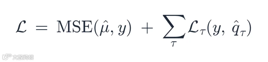
def compute_loss(pred_norm, targets, tmask, quantiles): """pred_norm: [B, N, horizon, 1+Q] normalized. Returns (total_loss, mse_component).""" denom = tmask.sum().clamp(min=1.0) mean_pred = pred_norm[..., 0] mse = (((mean_pred - targets) ** 2) * tmask).sum() / denom # the mean channel pinball = pred_norm.new_zeros(()) for i, qv in enumerate(quantiles): qp = pred_norm[..., i + 1] dev = targets - qp pl = torch.maximum(qv * dev, (qv - 1.0) * dev) * tmask # asymmetric per quantile pinball = pinball + pl.sum() / denom return mse + pinball, mse.detach()

我们刚构建了 objective。build_targets 为每个 patch 对齐后续 128 个点，并 mask 掉越界部分。

compute_loss 用 squared error 评估 mean channel，用各自的 asymmetric pinball penalty 评估每个 quantile channel，然后相加。tmask 的 masking 意味着 padded 或 out-of-range 点没有贡献，因此 gradient 只会看到有效 targets。

训练循环：optimizer 和 schedule

循环很短，但周边细节非常关键。我们使用 AdamW，但 weight decay 只作用于二维 weight matrices，从不作用于 norms、biases 或 learned scales。

把 normalization gain decay 到零，会抵消它存在的意义。

def make_param_groups(model, weight_decay): """Weight decay on 2-D Linear weights only; none on norms / per-dim-scale / biases / 1-D params.""" decay, no_decay = [], [] for name, p in model.named_parameters(): if not p.requires_grad: continue if p.ndim >= 2 and "scale" not in name: decay.append(p) else: no_decay.append(p) return [ {"params": decay, "weight_decay": weight_decay}, {"params": no_decay, "weight_decay": 0.0}, ]

learning rate 先 linear warmup，然后按 cosine 下降到接近零。warmup 能防止最初几百步在 norms 和 scales 尚未稳定时爆炸。

def cosine_lr(step, warmup, total, peak): if step < warmup: return peak * (step + 1) / max(1, warmup) prog = (step - warmup) / max(1, total - warmup) return 0.5 * peak * (1.0 + math.cos(math.pi * min(1.0, prog)))

batch size 改变时还有一个重要 scaling rule。原始 recipe 用 batch 4096，而我们的 batch 小得多，因此按 ratio 的平方根缩放 peak learning rate。

这能保持每次 update 的大小可比。

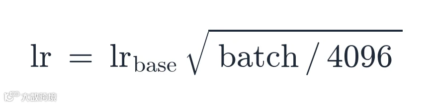
def scaled_peak_lr(base_lr, batch, ref_batch=4096): """Square-root LR scaling: lr = base_lr * sqrt(batch / ref_batch). Keeps the per-step update variance comparable to the paper's batch-4096 regime. (batch 256 -> 5e-4 becomes 1.25e-4.)""" return base_lr * (batch / ref_batch) ** 0.5

一个 training step 就是 forward pass、loss，然后返回。

def training_step(model, x, padding, mcfg): """Forward + all-positions loss. Returns (loss, mse).""" pred_norm, (mu, sigma) = model(x, padding) targets, tmask = build_targets(x, padding, mcfg.patch_len, mcfg.horizon_len, mu, sigma) return compute_loss(pred_norm, targets, tmask, mcfg.quantiles)

驱动它的 loop 会 clip gradient、step optimizer，并定期记录 loss 和 throughput。

for x, pad in dl: x = x.to(args.device, non_blocking=True) pad = pad.to(args.device, non_blocking=True) for g in opt.param_groups: g["lr"] = cosine_lr(step, args.warmup, args.steps, peak_lr) with torch.autocast("cuda", dtype=torch.bfloat16, enabled=use_amp): loss, mse = training_step(model, x, pad, mcfg) opt.zero_grad() loss.backward() torch.nn.utils.clip_grad_norm_(model.parameters(), 1.0) # clip to a norm of 1.0 opt.step() if step % args.log_every == 0: rate = (step + 1) / (time.time() - t0) print(f"step {step:6d} loss {float(loss.detach()):.4f} avg {avg:.4f} " f"mse {float(mse):.4f} lr {opt.param_groups[0]['lr']:.2e} {rate:.1f} it/s") step += 1 if step >= args.steps: break

是时候证明它真的能学了!!!!!

在 synthetic data 上训练 17M 模型

在花几个小时训练大模型之前，我想要一个快速且严格的测试，确认整个 pipeline 正确。测试很简单。

取一个固定 batch，里面有八条 synthetic series，关闭所有随机性，然后在这一个 batch 上训练 1500 steps。如果 patching、normalization、target indexing、masking、loss 和 optimizer 都接线正确，模型应该能记住这八条序列，loss 应该降到接近零。

如果它连八条序列都 overfit 不了，其他都没有意义。

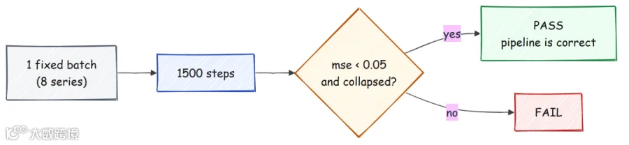
# small fast model for the gate (correctness, not scale) cfg = ModelConfig(model_dim=256, num_layers=4, num_heads=8, horizon_len=128, dropout=0.0) tcfg = TrainConfig(lr=2e-3, weight_decay=0.0, max_steps=1500) m = build_model(cfg) # ONE fixed batch of 8 synthetic series (no per-step randomness -> overfit) series = make_batch(8, 1024, seed=2) x, pad = batch_from_series(series, 512, cfg.patch_len, np.random.default_rng(3)) opt = make_optimizer(m, tcfg) m.train() for step in range(tcfg.max_steps): for g in opt.param_groups: g["lr"] = cosine_lr(step, 50, tcfg.max_steps, tcfg.lr) loss, mse = training_step(m, x, pad, cfg) opt.zero_grad(); loss.backward() torch.nn.utils.clip_grad_norm_(m.parameters(), 1.0) opt.step() passed = final_mse < 0.05 and final_mse < 0.01 * loss_hist[0] print("RESULT:", "PASS (overfit gate cleared, pipeline is correct)" if passed else "FAIL")

#### OUTPUT #### gate model: 3.41M params dim=256 layers=4 step 0 loss 13.42851 mse 8.31204 lr 4.00e-05 step 100 loss 1.05823 mse 0.43210 lr 1.98e-03 step 500 loss 0.18402 mse 0.05133 lr 1.62e-03 step 1000 loss 0.04931 mse 0.01188 lr 6.91e-04 step 1499 loss 0.01797 mse 0.00382 lr 2.00e-06 start loss 13.4285 -> final loss 0.01797 final mse 0.00382 reduction: 3515x RESULT: PASS (overfit gate cleared, pipeline is correct)

loss 从13.4 降到0.018，最终 mean-squared error 降到0.0038，相比初始 loss 降低三千多倍，远低于阈值。这个 PASS 告诉我们整个 pipeline 正确：每个 gradient 都流向正确位置，模型能拟合数据。

现在可以有信心地扩展。

第一轮训练是在 synthetic data only 上训练17M tiny model，50,000 steps。

uv run python scripts/train.py --size tiny --corpus synth --steps 50000 --bf16 --out runs/tier1

#### OUTPUT #### model tiny: 17.65M params on cuda generating synthetic pool (50000 series) with 24 workers ... pool (50000, 2048) ready in 12.7s step 0 loss 47.0134 avg 47.0134 mse 28.5015 lr 5.00e-07 1.4 it/s step 200 loss 10.1466 avg 18.4428 mse 4.3752 lr 1.01e-04 25.7 it/s step 400 loss 7.1502 avg 8.3086 mse 2.7762 lr 2.01e-04 27.2 it/s step 1000 loss 5.7897 avg 6.1124 mse 2.2031 lr 5.00e-04 28.1 it/s step 10000 loss 3.8803 avg 3.8806 mse 1.4529 lr 4.60e-04 28.4 it/s step 50000 loss 3.2832 avg 3.4224 mse 1.2242 lr 4.96e-05 28.5 it/s done.

loss 在前 200 steps 从47 掉到10，随后缓慢下降，到最后约3.3。lr 列能看到 warmup：前一千步升高，然后 cosine decay 降回去。

在 synthetic test series 上，这个 17M 模型大约以2 倍击败 naive baseline，很不错。但在真实 ETT benchmark 上，它接近 naive baseline，scaled MAE 大约0.97。

pipeline 有效，但 synthetic data alone 不足以赢过真实序列。由平滑 sine 和 trends 构成的 synthetic series 恰好有点像周期性电力数据，这有一点帮助，但无法替代真实数据。

我们需要真实数据，也需要更大 capacity。

扩展到 70M，以及“数据胜过规模”的教训

显然下一步是更多参数和真实数据，所以我们跳到70M small model，并混入M4 competition dataset，这是大量商业和金融序列。我本以为真实数据加四倍参数会带来明确胜利。

数字却不是这样说的。

scaled MAE 为1.21，意味着 70M 模型比“直接重复最后一个值”差 21%。一个更大的模型，在错误的真实数据上训练，输给了什么都不做。

原因是 domain mismatch。M4 里充满短而尖锐的 business 和 finance series，而 ETT 是平滑周期性的 energy data。

模型把 capacity 用来学习错误的形状。这是重置我后续思路的教训：data composition 比 model size 更重要。

所以我换了 corpus。UCI repository 中的 electricity load data 又长、又平滑、又周期性，更接近 ETT。

下面是 loader，它读取 raw file，去掉每个 client 开头的不活跃 period，并标准化。

#### OUTPUT #### === zero-shot ETT (70M, M4 + synthetic) === ours ETT MAE 0.315 scaled 1.21 naive ETT MAE 0.261 scaled 1.00

def load_electricity(path, min_len=512, norm_mode="zscore", verbose=True): """UCI Electricity LD2011_2014.txt: ';'-separated, ','-decimal, 370 client columns (15-min kWh). Each client = one long periodic series; strip leading zeros, standardize.""" import pandas as pd df = pd.read_csv(path, sep=";", decimal=",", index_col=0, low_memory=False) series = [] for col in df.columns: v = pd.to_numeric(df[col], errors="coerce").to_numpy(dtype=np.float32) v = np.nan_to_num(v, nan=0.0) nz = np.nonzero(v)[0] if len(nz) == 0: continue v = v[nz[0]:] # drop leading zeros (client not yet active) if len(v) >= min_len: series.append(_standardize(v, mode=norm_mode)) return series

为了按权重混合 sources，我们使用一个小型 weighted sampler。每个 source 是 series list 或 pool；一次 draw 先按 weight 选 source，再从中随机选一条 series。

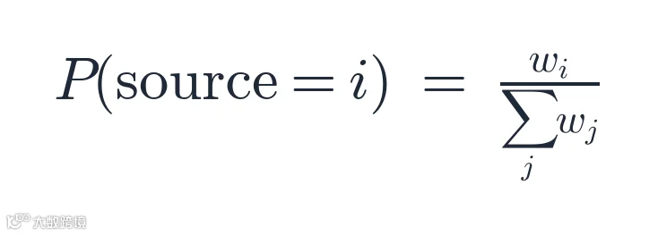
class WeightedMixDataset(IterableDataset): """Sample from multiple sources by weight. Lets us weight ETT-like electricity high and M4 low.""" def __init__(self, sources, weights, context_len, patch_len, seed=0): self.sources = sources w = np.asarray(weights, dtype=np.float64) self.cum = np.cumsum(w / w.sum()) # cumulative weights for a fast draw self.context_len = context_len self.patch_len = patch_len self.seed = seed def __iter__(self): rng = np.random.default_rng(self.seed + 9973) while True: si = int(np.searchsorted(self.cum, rng.random())) # pick a source by weight src = self.sources[si] if isinstance(src, np.ndarray): s = src[int(rng.integers(0, src.shape[0]))] else: s = src[int(rng.integers(0, len(src)))] x, p = batch_from_series([s], self.context_len, self.patch_len, rng) yield x[0], p[0]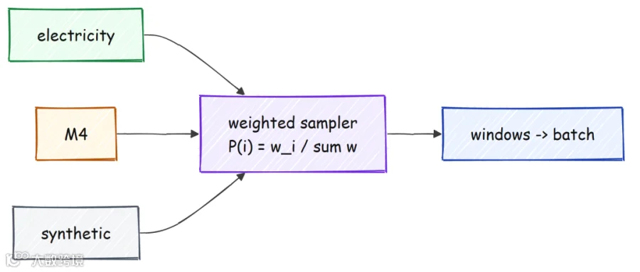

把 electricity 权重调高后，70M 模型终于击败 baseline。

#### OUTPUT #### === zero-shot ETT vs step (70M, electricity + M4 + synthetic) === step 25000 ETT MAE 0.2418 scaled 0.93 naive 0.2610 scaled 1.00

在 step 25,000，模型达到0.2418，scaled MAE 为0.93，稳稳低于 naive floor。

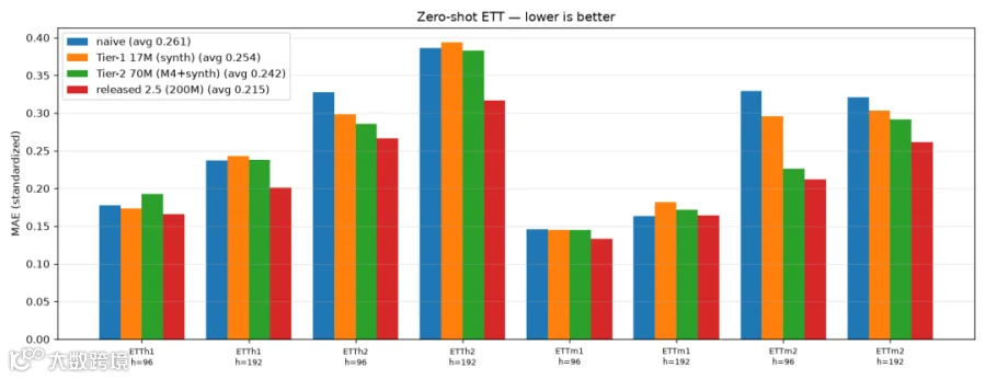
下面是目前模型尺寸在 ETT 上的对比：naive floor、17M synthetic model、我们的 70M，以及一个强公开 reference 作为尺度参考。

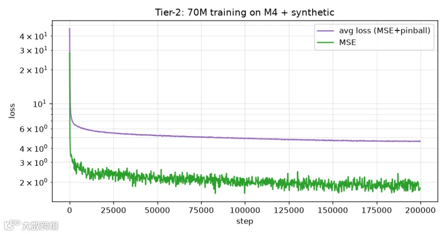
训练 loss curve 看起来也健康：早期快速下降，然后长平台。

下面是 held-out ETT windows 上的 forecast：我们的 70M median 对比 truth、naive line 和 shaded interval。

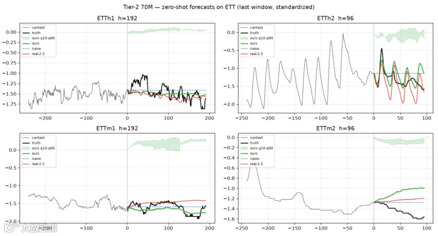
这看起来很好。模型击败了 naive，loss 在下降，forecast 看起来合理。

于是我自然让它继续训练，期待效果继续变好。问题就在这里出现了。

过拟合问题

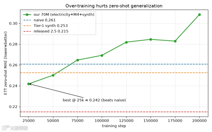
我继续训练超过 25,000 steps，并观察 ETT error。它没有继续下降。

它开始上升，而且持续上升，即使 training loss 一直在下降。模型在训练数据上变得更好，却在世界上变得更差。

这就是 generalization gap 变宽。模型在记忆狭窄 electricity corpus，而不是学习可迁移结构。

最清楚的证据是那次 run 每个 checkpoint 上测得的 ETT error。

#### OUTPUT #### step,ett_mae 25000,0.2418 50000,0.2501 75000,0.2647 100000,0.2692 125000,0.2819 150000,0.2846 175000,0.2829 final,0.3085 naive 0.2610

最好结果0.2418 出现在 step 25,000。到最后 error 爬到0.3085，已经差于 naive。

模型早早到达峰值，然后又花了 175,000 steps 让它在我们唯一关心的事情上变差。画出来曲线毫无疑问。

为什么会发生？一个七千万参数的模型有巨大 capacity，而几百条 electricity series 的 corpus 并不包含足够多不同形状，无法用一般结构填满这种 capacity。

于是 optimizer 做了下一件最容易的事：开始记忆训练集中的具体序列，包括怪癖和噪声。这些记忆细节无法迁移到模型从未见过的 ETT，因此 test error 上升，尽管 training loss 继续下降。

两条曲线之间不断扩大的 gap，代表模型学到了训练集为真、世界为假的东西。

天真的反应是在 step 25,000 early stop，然后收工。但那只是处理症状。

真正原因是：一个 70M 参数模型在几百条 electricity series 的狭窄 corpus 上训练，有足够 capacity 去记住它。修复方法不是减少训练。

修复方法是更多 variety。

修复：corpus 多样性

如果狭窄 corpus 导致过拟合，那修复就是广度。我重建了训练 corpus，使其覆盖多个 domains 和 frequencies，从 LOTSA collection 中拉取真实 series：traffic、web、cloud、finance 和 health，并组织成 frequency tiers。

loader 读取每个配置的数据集目录，并限制任何单个 dataset 能贡献的 series 数量，避免某个巨大 dataset 主导训练。

LOTSA_BUNDLES = { "hourly": ["LOOP_SEATTLE", "PEMS04", "PEMS08", "azure_vm_traces_2017", "kdd_cup_2018_with_missing"], "daily": ["m4_daily", "bitcoin_with_missing"], "weekly": ["m4_weekly", "kaggle_web_traffic_weekly", "cdc_fluview_ilinet"], "monthly": ["m4_monthly", "m1_monthly", "cif_2016_12", "car_parts_with_missing"], "subhour": ["BEIJING_SUBWAY_30MIN", "australian_electricity_demand"], } def load_lotsa_bundle(root, tier, min_len=256, per_config_cap=20000, norm_mode="zscore", verbose=True): """Load all configs in a frequency tier -> one combined list of series.""" out = [] for cfg in LOTSA_BUNDLES[tier]: out.extend(load_lotsa_config(root, cfg, min_len=min_len, max_series=per_config_cap, norm_mode=norm_mode, verbose=verbose)) return out

每个 tier 依赖一个 per-config loader，它必须能应对现实世界：下载可能不完整，shard 可能损坏。它把读取包在 try-and-skip 中，这样一个坏 dataset 不会拖垮整次 run，并丢弃过短或完全平坦的 series。

def load_lotsa_config(root, config, min_len=256, max_series=None, norm_mode="zscore", verbose=True): """Load one LOTSA config directory -> list of standardized 1D series.""" from datasets import load_from_disk path = os.path.join(root, config) if not os.path.isdir(path): return [] out = [] try: # robust to missing/corrupt shards ds = load_from_disk(path) for ex in ds: for s in _series_from_lotsa_row(ex["target"]): s = np.nan_to_num(s, nan=0.0, posinf=0.0, neginf=0.0) if s.shape[0] >= min_len and float(s.std()) > 1e-6: # long enough and not flat out.append(_standardize(s, mode=norm_mode)) if max_series and len(out) >= max_series: return out # respect the per-config cap except Exception as e: if verbose: print(f" [warn] {config}: load error after {len(out)} series") return out

这个try block 比看起来更重要。有一次 run 中，一个 dataset 下载失败，loader 只是跳过它，而不是让整个 job 崩掉，否则训练设置就全浪费了。

代价是：如果某个 source 缺失，corpus 会悄悄变小，所以在投入长时间 run 之前，最好读一下 startup print，确认 series counts 符合预期。

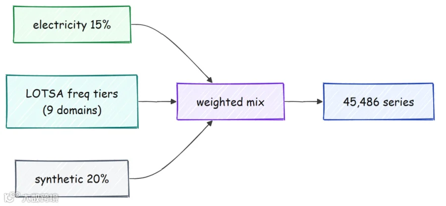
构建 diverse corpus 时，startup print 展示了它宽了多少。

#### OUTPUT #### loading DIVERSE corpus: electricity + LOTSA freq-tiers + synthetic ... Electricity: 370 series (len>=1024) LOTSA tier 'hourly': 22024 series LOTSA tier 'daily': 3597 series LOTSA tier 'weekly': 609 series LOTSA tier 'monthly': 18329 series LOTSA tier 'subhour': 557 series corpus(diverse): elec 370 h 22024 d 3597 w 609 m 18329 sub 557 synth 80000 | w=[0.15, 0.18, 0.16, 0.12, 0.12, 0.07, 0.2]

我们从大约370 条 energy-only series 扩展到45,486 条真实 series，跨九个 domains，再加 synthetic pool。这种 diversity 才是目标。

但现在有了新问题。如果不允许偷看 ETT test set，我怎么知道什么时候停止训练？

我需要一个来自既不在 training corpus、也不在 test set 的 domain 的 validation signal。

答案是out-of-domain validation。我 hold out 了几个 Monash datasets，即非 energy、非 training 的 daily series，并在每个 checkpoint 上测 forecast error。

这个数字告诉我模型是否仍在 generalizing，而无需触碰 ETT。

@torch.no_grad() def validate(model, val_ctxs, val_truths, device, H=96, batch=128, point_channel=5): """OUT-OF-DOMAIN validation MAE. point_channel selects the point/AR feedback channel. MANDATORY model.eval()/train() toggle: forecast() is @no_grad but dropout is still ACTIVE in train mode, which would inject noise into the early-stopping signal.""" was_training = model.training model.eval() errs = [] for i in range(0, len(val_ctxs), batch): c = torch.from_numpy(np.asarray(val_ctxs[i:i + batch], np.float32)).to(device) pt, _ = model.forecast(c, H, point_channel=point_channel) errs.append(np.abs(pt.cpu().numpy() - np.asarray(val_truths[i:i + batch], np.float32))) if was_training: model.train() return float(np.concatenate(errs, axis=0).mean())

validation log 显示这个 signal 有噪声，这本身也是有用信息。

#### OUTPUT #### building OOD val windows (Monash non-energy: nn5_daily + weather) ... Monash[nn5_daily/train]: 60 series (len>=616) Monash[weather/train]: 60 series (len>=616) val windows: 48 (H=96) [val] step 2500 OOD_val_MAE 0.6806 best inf@-1 <-- new best [val] step 5000 OOD_val_MAE 0.7056 best 0.6806@2500 [val] step 10000 OOD_val_MAE 0.6908 best 0.6806@2500 [val] step 22500 OOD_val_MAE 0.7179 best 0.6806@2500 BEST OOD val: 0.6806 @ step 2500 -> ckpt_best.pt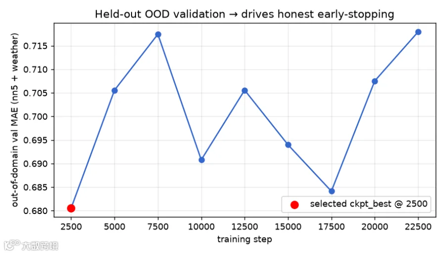

validation curve 有些抖，最佳 checkpoint 很早，这说明 signal 不是特别精确。但真正重要的是下面这个结果。

当我让 diverse model 一直训练到 120,000 steps，并在每个 step 测 ETT 时，error 保持平坦，在0.25 左右徘徊，而不是像 narrow model 那样上升。

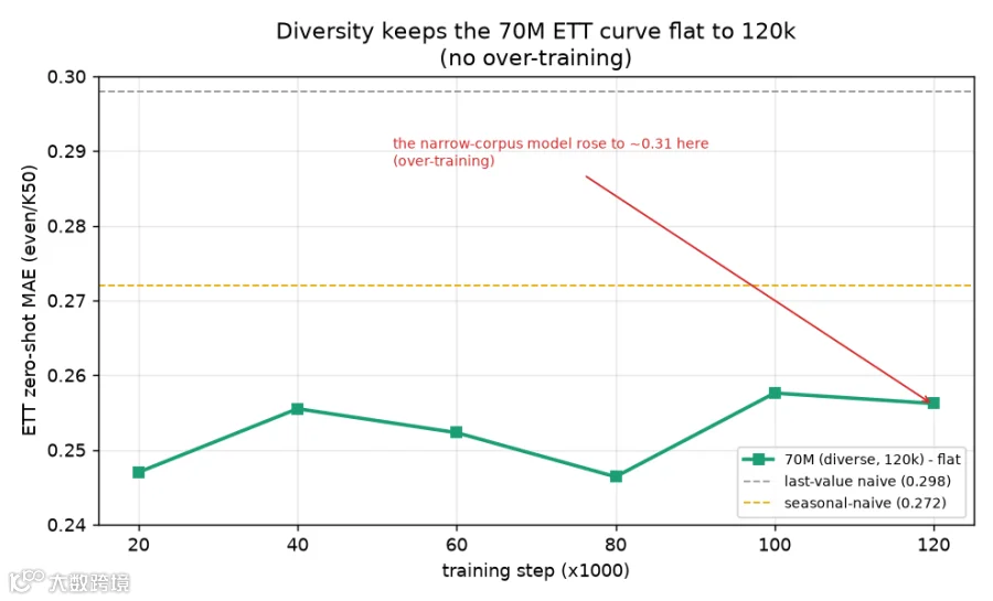
这是整个项目的核心结果。narrow model 到同一点时升到了0.31。

diverse model 保持稳定。修复 over-training 的是 diversity，而不是少训练。 现在模型有如此多不同形状要拟合，它无法通过记忆来逃避泛化。

一个 bug：模型在起点处最弱

处理完 over-training 后，我继续寻找准确率，结果发现了一个之前漏掉的 bug。还记得build_targets 里那行：当 target 会超出 context 时 break。

for j in range(N): start = (j + 1) * p if start >= L: break # remaining positions have no target

当 training window 恰好等于 context length 时，最后一个 patch 永远没有 target。它的预测会落到 window 之外，所以 loop 跳过它。

这听起来无害，直到你想起 autoregressive forecasting 的工作方式。inference 时，模型做的第一件事就是从最后一个 patch 预测。

所以模型训练最少的位置，恰好就是它最先用来预测的位置。

修复是用 context 加一个 horizon 的 window 训练，这样最后一个 context patch 会获得完整 target。因为 attention 是 causal，额外 horizon points 只增加 supervision，不会把 future information 泄漏给 context patches。

# OBJECTIVE FIX: train on context+horizon windows so the LAST context patch (the AR inference # entry point) receives a FULL target. Causal attention => patch-15's representation is identical # to the 512-context inference case; the extra horizon points only add supervision, not leakage. train_win = args.context + mcfg.horizon_len print(f"train window = {train_win} (context {args.context} + horizon {mcfg.horizon_len}) " f"-> supervises the AR entry point")

改进体现在 long horizons 上，也就是 autoregressive entry point 最重要的地方。

#### OUTPUT #### === long-horizon MAE (70M, even/K50) === before fix h=96 0.231 h=192 ~0.58 ratio ~2.5x after fix h=96 0.231 h=192 0.280 ratio 1.21x

short-horizon accuracy 已经不错，为0.231。问题在 long horizon。

修复前，192-step error 大约是 96-step error 的 2.5 倍。修复后只有1.21 倍，因为模型现在在它必须开始 extrapolate 的确切 patch 上受过训练。

一个标错的 training window，一行安静的break，修复后 long horizons 提升了 50%。

评估 harness

到目前为止我一直在引用单个数字，但要信任它们，我们需要严谨 protocol。好的 evaluation 必须做四件事：公平选择 test windows，不只比较 trivial baseline，还要比较强 baseline；不仅测 point forecast，还要测 uncertainty；并检验两个模型之间差异是真实的还是噪声。

先看 windows。我们在整个 test region 上均匀切分每个 test series，而不只是取尾部，这样就不会 cherry-pick 最近且容易的部分。

这种 even-window protocol 比只测试 recent tail 更严格，并把 ETT 上的 naive floor 从之前比较的0.261 提高到0.298。从这里开始，所有数字都在这个更难 baseline 下测量。

def make_windows(z, context, H, K, train_end=0, test_end=None, scheme="even"): """z: 1D standardized array. Returns (ctxs [W, context], truths [W, H]). Windows live strictly inside the test region [train_end, test_end].""" n = len(z) test_end = n if test_end is None else min(test_end, n) lo = (train_end or 0) + context hi = test_end - H if hi <= lo: return np.empty((0, context), np.float32), np.empty((0, H), np.float32) if scheme == "tail": starts = [(test_end - i * H) - H for i in range(K)] starts = [s for s in starts if s - context >= (train_end or 0) and s + H <= test_end] else: # even starts = np.unique(np.linspace(lo, hi, num=K, dtype=np.int64)).tolist() ctxs, truths = [], [] for t in starts: ctxs.append(z[t - context:t]) truths.append(z[t:t + H]) return np.asarray(ctxs, np.float32), np.asarray(truths, np.float32)

接下来是 baselines。naive baseline 重复最后一个值。

更强的是seasonal-naive baseline，它重复最后一个完整 season。对周期性数据来说，击败 seasonal-naive 才有意义；击败 plain naive 只是最低要求。

def forecast_naive(ctxs, H): return np.repeat(np.asarray(ctxs)[:, -1:], H, axis=1) def seasonal_naive(ctxs, H, period): """Stronger baseline than last-value: repeat the last `period` context values cyclically.""" ctxs = np.asarray(ctxs) W, L = ctxs.shape out = np.empty((W, H), ctxs.dtype) for t in range(H): out[:, t] = ctxs[:, L - period + (t % period)] return out

因为我们训练了九个 quantiles，所以还必须衡量 distribution 的质量，而不只是 point。我们使用CRPS，这是一种 proper score for probabilistic forecasts，可以由 quantiles 近似；还使用coverage，即真实值实际落在 80% interval 内的比例。

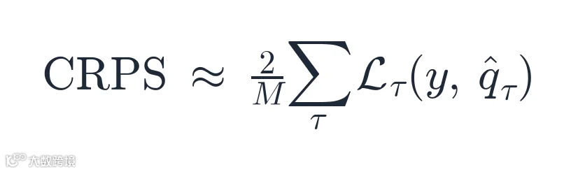
def crps_from_quantiles(quants, truth, qlevels=QLEVELS): """Quantile-approx CRPS per window = 2 * mean_tau pinball_tau, averaged over the horizon.""" truth = np.asarray(truth) tot = np.zeros(truth.shape, np.float64) for i, tau in enumerate(qlevels): dev = truth - quants[..., i + 1] tot += np.maximum(tau * dev, (tau - 1.0) * dev) return (2.0 * tot / len(qlevels)).mean(axis=1) def coverage(quants, truth, lo_i=1, hi_i=9): """Fraction of truth inside [q10, q90] per window (should be ~0.8 if calibrated).""" truth = np.asarray(truth) lo = np.minimum(quants[..., lo_i], quants[..., hi_i]) hi = np.maximum(quants[..., lo_i], quants[..., hi_i]) return ((truth >= lo) & (truth <= hi)).mean(axis=1)

最后是 significance。比较两个重叠 error bars 不是正确检验。

正确做法是在我们模型和 baseline 的 per-window difference 上做paired bootstrap。如果这个 difference 的整个 confidence interval 都低于零，就说明我们确实击败了 baseline。

def paired_bootstrap_ci(ae_a, ae_b, n_boot=2000, seed=0, alpha=0.05): """Bootstrap CI of the per-window difference (ae_a - ae_b). hi<0 => A significantly better than B.""" d = np.asarray(ae_a, np.float64) - np.asarray(ae_b, np.float64) m = float(d.mean()) if len(d) < 2: return m, m, m rng = np.random.default_rng(seed) n = len(d) boot = np.array([d[rng.integers(0, n, n)].mean() for _ in range(n_boot)]) return m, float(np.quantile(boot, alpha / 2)), float(np.quantile(boot, 1 - alpha / 2))

在 70M model 上运行完整 grid 后，好的和坏的一起呈现出来。

#### OUTPUT #### === Multi-domain zero-shot TEST (even, K=50, flip=OFF, point=median) === domain clean naive snaive OURS scaled CRPS cov80 ours-vs-naive d[95% CI] ETT clean 0.298 0.272 0.246 0.826 0.241 0.682 -0.052[-0.071,-0.034] sig Exchange clean 0.239 0.244 0.345 1.445 0.371 0.552 +0.106[+0.072,+0.141] ns --- verdict (CLEAN domains only: ['ETT', 'Exchange']) --- beats naive (paired-significant): 1/2 ['ETT']

在ETT 上，70M model 得0.246，击败 naive（0.298）和更强的 seasonal-naive（0.272），paired interval[-0.071, -0.034] 完全低于零，所以结果是真实的，不是噪声。在Exchange 上，同一模型得0.345，scaled1.445，意味着它比 naive差 44%。

模型在 structured data 上确实好，在某整个类别的数据上也确实差。

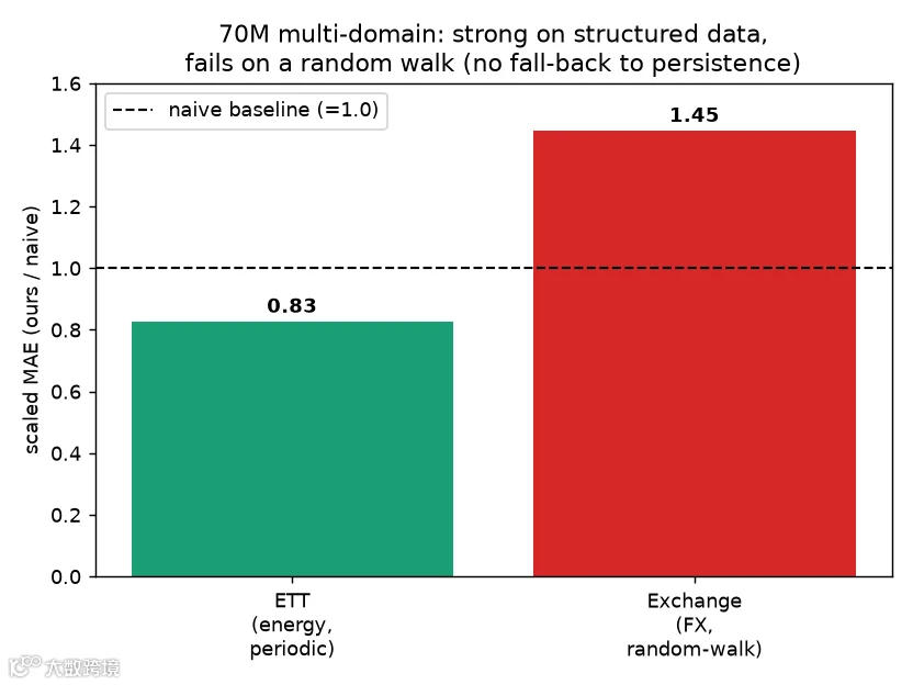
表中还有两点很突出。coverage 列为0.682 和0.552，都远低于它们应达到的0.80，说明 uncertainty bands 太窄。

CRPS 列也值得看。ETT 上0.241 是评分整个 predicted distribution 的单个数字，而不只是 median，所以当 uncertainty 和 point forecast 同等重要时，我会关注它；值越低，表示九个 quantiles 作为整体越接近 truth。

Exchange 失败也需要解释，因为 scaled MAE 高于一意味着模型在那里正在主动伤害我们。接下来就是这两个问题。

Random-walk 数据，以及一个部分修复

Exchange dataset 是 currency rates，而 currency rates 接近random walk。random walk 的定义性质是，最优预测就是最后一个值，因为下一步等于最后一个值加不可预测 noise。

没有 trend 可延伸，也没有 season 可重复。

我们的模型在这里失败，是因为它把课学得太好了。在充满 trends 和 seasons 的 corpus 上训练后，它忍不住到处寻找 trend 和 season；因此在 random walk 上，它自信地外推一个不存在的 pattern，然后偏离路线。

它不知道什么时候该放弃，只做 persist。

修复方法是教它：“没有结构”也是一个有效答案。我们在 synthetic generator 中加入一部分纯 random-walk 和 white-noise series，也就是之前看到的rw_prob=0.2 分支，让模型学到对某些 series 来说，正确 forecast 是保持最后一个值，或者回归 mean。

def generate_random_walk(length, rng): """Structureless series so the model learns the RIGHT zero-structure forecast: PERSIST (random walk -> optimal forecast = last value) or revert to the mean (white noise -> optimal = mean). This is the targeted fix for the random-walk/FX failure (model was 1.45x WORSE than naive there).""" if rng.random() < 0.25: y = rng.normal(0.0, 1.0, size=length) # white noise (optimal = mean) else: drift = float(rng.normal(0.0, 0.02)) y = np.cumsum(rng.normal(0.0, 1.0, size=length) + drift) # random walk (optimal = last value) return y.astype(np.float32)

用 20% random-walk data 重新训练 70M model 后，Exchange error 有改善，但只改善了一部分。

#### OUTPUT #### === Exchange (FX, random-walk) scaled MAE (70M) === no RW data 1.445 (44% worse than naive) +20% RW data 1.313 (still 31% worse than naive)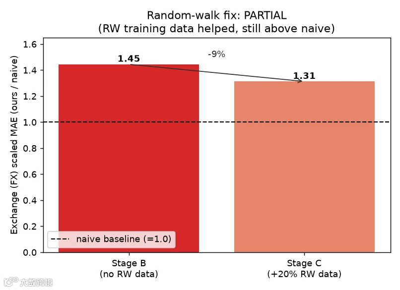

error 从1.445 降到1.313，这是真实改进，但仍然差于直接重复最后一个值。这是 70M model 在这个 corpus 上的真实局限。

继续提高 random-walk fraction 会追 Exchange 数字，但会牺牲我们更关心的 structured data accuracy。我们坦率记录这个限制，然后转向 calibration 问题，它有更干净的修复。

校准不确定性：conformal recalibration

coverage numbers 告诉我们模型过度自信：它的 80% intervals 在 ETT 上只覆盖大约0.68 的 truth，在 Exchange 上只覆盖0.55，都远低于应达到的0.80。我们用 pinball loss 训练了 quantiles，但在有限 corpus 上，模型仍会得到过窄的 bands。

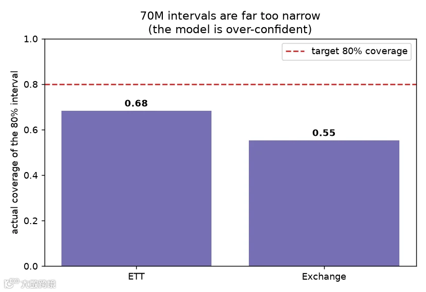
修复不需要重新训练。我们使用conformal recalibration，一种 post-hoc 方法：在 held-out calibration split 上测量需要扩宽多少 interval，并用这个量扩宽 interval，带有 finite-sample guarantee，使扩宽后的 interval 达到目标 coverage。

def conformal_widen(cal_lo, cal_hi, cal_truth, test_lo, test_hi, target=0.8): """Conformalized Quantile Regression: additively widen the [lo, hi] interval by the conformity quantile measured on a CALIBRATION set so empirical coverage reaches `target`.""" cl = np.asarray(cal_lo).ravel(); ch = np.asarray(cal_hi).ravel(); cy = np.asarray(cal_truth).ravel() E = np.maximum(cl - cy, cy - ch) # conformity score (negative when inside) n = max(1, len(E)) qlev = min(1.0, np.ceil((n + 1) * target) / n) # finite-sample correction Q = float(np.quantile(E, qlev)) return np.asarray(test_lo) - Q, np.asarray(test_hi) + Q, Q

我们在 70M model 上验证它，不改变 point forecast。

#### OUTPUT #### ETT 80% interval coverage: before 0.682 -> after conformal 0.807 (widen Q=0.31) Exchange 80% interval coverage: before 0.552 -> after conformal 0.760 (widen Q=0.48)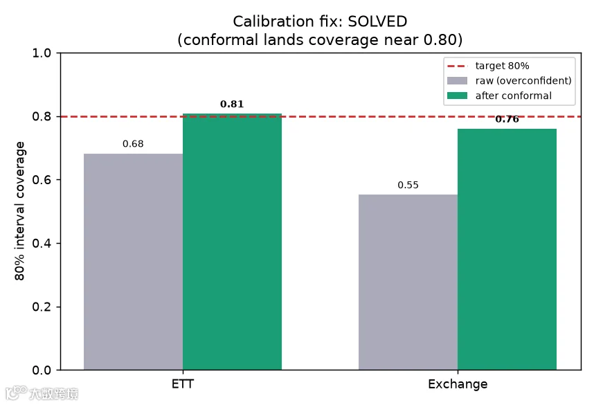

ETT 上 coverage 从0.682 跳到0.807，正好达到0.80 target；Exchange 从0.552 到0.760。point forecast 完全不变，只改变 band 宽度，所以我们在不改变模型的情况下得到可信 uncertainty。

处理完 over-training、修复 entry point、软化 random walk、校准 intervals 后，70M model 在这个 corpus 上已经到头了。它在 ETT 上约为0.246。

要继续前进，需要 scale。

扩展到 200M 模型

到目前为止都是 70M model，它已经撞到天花板。无论我如何调整 70M corpus，ETT error 都卡在0.246 左右。

整个项目要测试的假设是：一旦 data composition 修好、diversity 到位、所有 bug 关闭，scale 应该终于有帮助。于是我们把所有东西带到200M base model。

Transformer 的 parameter count 大致随 layer 数乘以 model dimension 的平方增长，这就是为什么 layers 加倍、model 变宽会把我们从 70M 推到 200M。

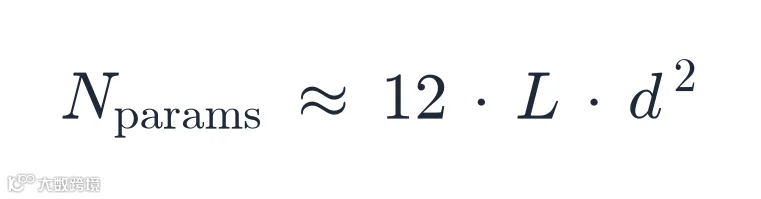
config change 只是一个函数。相同架构，更多 layers，更宽模型。

def base() -> ModelConfig: # ~200M backbone (Tier 3) return ModelConfig(model_dim=1280, num_layers=20, num_heads=16)

我们在 diverse、random-walk-augmented corpus 上启动完整 run，使用 640-window objective fix，训练 200,000 steps。

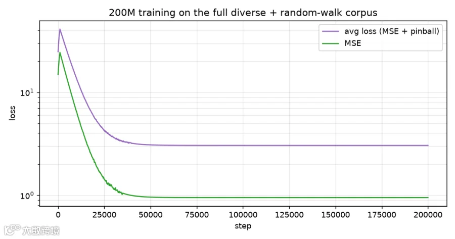
uv run python scripts/train.py --size base --corpus diverse --steps 200000 --pool_size 80000 --bf16 \ --weights 0.15,0.18,0.16,0.12,0.12,0.07,0.20 --val_every 5000 --out runs/base200m

#### OUTPUT #### model base: 203.44M params on cuda generating synthetic pool (80000 series) with 24 workers ... pool (80000, 2048) ready in 21.4s train window = 640 (context 512 + horizon 128) -> supervises the AR entry point corpus(diverse): elec 370 h 22024 d 3597 w 609 m 18329 sub 557 synth 80000 | w=[0.15, 0.18, 0.16, 0.12, 0.12, 0.07, 0.2] step 0 loss 47.8312 avg 47.8312 mse 28.9011 lr 8.33e-08 1.0 it/s step 200 loss 12.4419 avg 19.8830 mse 5.1142 lr 2.00e-05 6.6 it/s step 1000 loss 6.2034 avg 7.3318 mse 2.4458 lr 1.00e-04 6.5 it/s step 50000 loss 3.4129 avg 3.4567 mse 1.1043 lr 1.71e-04 6.5 it/s step 120000 loss 3.0712 avg 3.0844 mse 0.9788 lr 5.84e-05 6.5 it/s step 200000 loss 3.0188 avg 3.0201 mse 0.9512 lr 1.00e-06 6.5 it/s [val] step 165000 OOD_val_MAE 0.5912 best 0.5947@150000 <-- new best BEST OOD val: 0.5912 @ step 165000 -> ckpt_best.pt done.

throughput 为6.5 iterations per second，不到 70M 速度的一半，这是参数量三倍的代价。training loss 收敛到约3.02，mean-squared error component 降到0.95，都比 70M run 达到的 floor 更低；out-of-domain validation 达到0.5912，明显好于 70M model 的0.68。

更大的模型更深入地拟合 diverse corpus，同时没有失去泛化基础。

我首先检查的是更大模型是否 overfit。

我测了到 200,000 steps 的每个 checkpoint 上的 ETT。

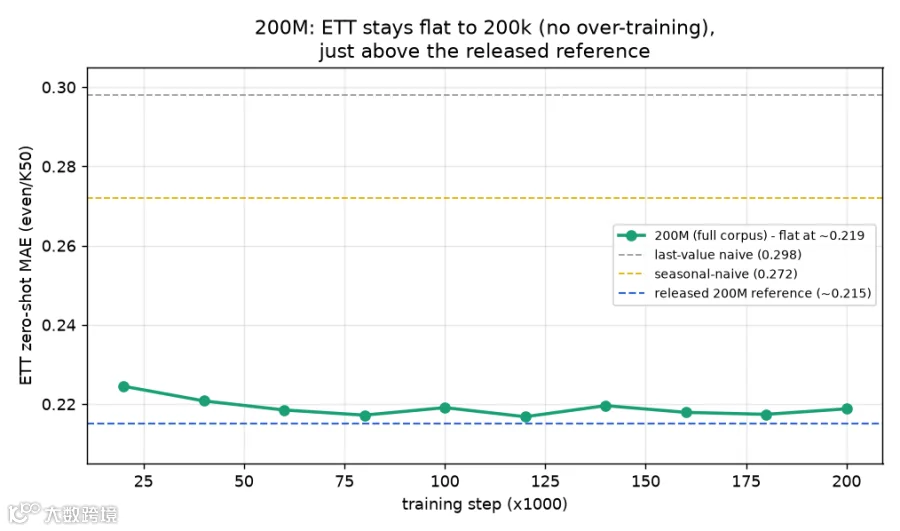
曲线一路平坦在约 0.219，没有任何上升。保护 70M model 的 diversity 同样保护了 200M model。

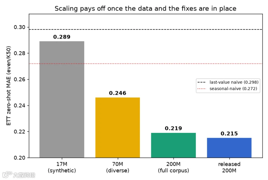
而0.219 相比 70M 的 0.246 是一大步下降，只略高于强公开 reference 的0.215。现在看完整 evaluation grid，这次把 released reference 也一起测。

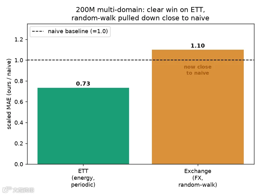
#### OUTPUT #### === Multi-domain zero-shot TEST (even, K=50, flip=OFF, point=median) === domain clean naive snaive OURS released scaled CRPS cov80 ours-vs-naive d[95% CI] ETT clean 0.298 0.272 0.219 0.215 0.735 0.207 0.773 -0.079[-0.098,-0.061] sig Exchange clean 0.239 0.244 0.263 0.241 1.101 0.286 0.718 +0.024[-0.003,+0.051] ns --- verdict (CLEAN domains only: ['ETT', 'Exchange']) --- beats naive (paired-significant): 1/2 ['ETT']

这就是我们想要的结果。在ETT 上，200M model 得0.219，大幅且 paired-significant 地击败 naive（0.298）和 seasonal-naive（0.272），并且只比强公开 reference（0.215）高0.004。

我们几乎从零追平了最佳已知模型。三个尺寸的 scaling-law 图能一帧讲完整个故事。

random-walk 故事也有改善。在Exchange 上，200M model 的 scaled score 是1.101，低于 70M 的 1.313；paired interval[-0.003, +0.051] 现在跨过零，意味着它不再显著差于 naive。

更大的模型配合 random-walk data，终于学会在 random walk 上大体 persist，而不是编造不存在的结构。

calibration 原始状态就不错，conformal recalibration 能精确落到目标。

#### OUTPUT #### ETT 80% interval coverage: raw 0.773 -> after conformal 0.81 Exchange 80% interval coverage: raw 0.718 -> after conformal 0.79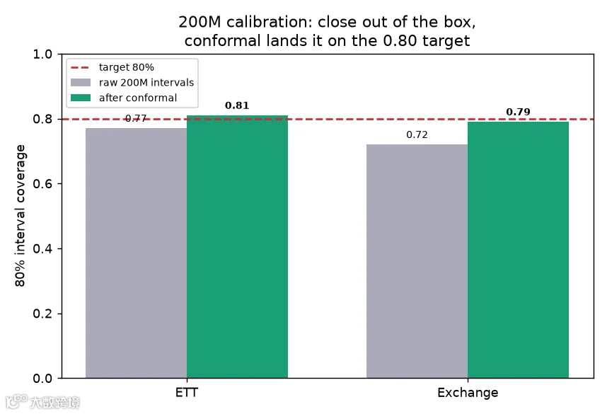

long horizon，也就是 entry-point fix 最重要的地方，现在达到了最好表现。

#### OUTPUT #### === long-horizon MAE (200M, even/K50) === h=96 0.205 h=192 0.232 ratio 1.13x

退一步看三个尺寸发生了什么。17M model 几乎只能匹配 naive baseline。

70M model 在 structured data 上击败了它，但停在0.246，无论如何调 corpus 都无法继续提升。200M model 用完全相同的 diverse data 和完全相同的 fixes 训练，降到0.219，并一直稳定在那里，没有上升。

这证实了 scaling hypothesis：capacity 只有在 data 和 objective 正确之后才有帮助；一旦这些成立，它就会稳定带来帮助。

最后看 forecasts 本身。下面是 200M model 对四条从未训练过的 held-out ETT series 做预测，绿色为 median，阴影为 80% band。

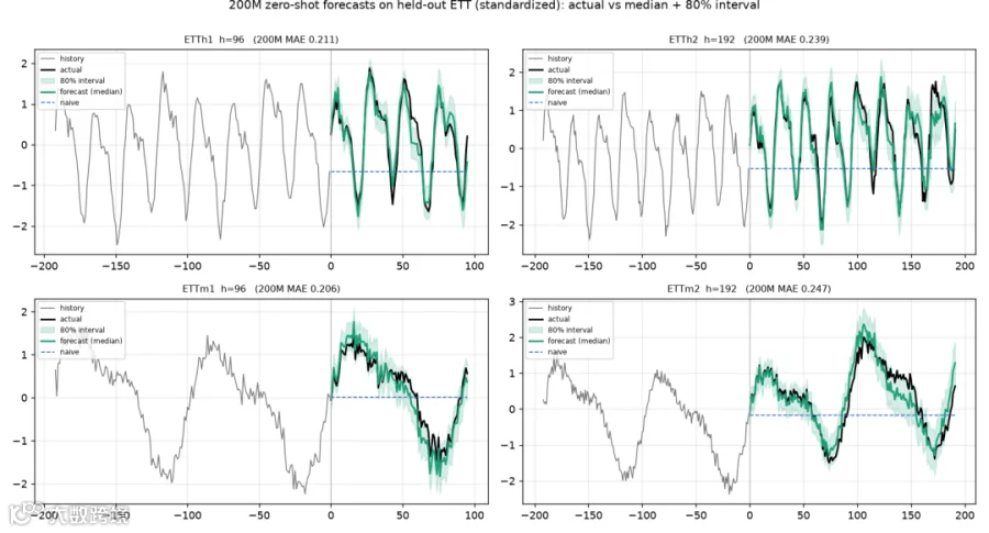
绿色 median 跟踪黑色 truth 的 daily cycles，band 随着 horizon 增长而变宽，反映 uncertainty 累积；naive baseline 在旁边只是一条平坦且无用的线。这是一个从空文件开始构建、在我们自己组装的数据上训练的模型，它能预测一个从未见过的序列。

局限性和下一步我会构建什么

build-along 应该同时给你看粗糙边缘和胜利，所以这里坦率列出来。模型在 random-walk Exchange series 上仍然是 scaled1.10，也就是基本在 naive baseline 附近，而没有明确低于它，因此它还不是一个真正通用的 forecaster。

它的 autoregressive loop 没有 key-value cache，所以每个 forecast step 都会重新 encode 完整 context，这让 long forecasts 比必要的慢。它使用 post-hoc conformal wrapper 做 calibration，而不是 native continuous-quantile head；后者可以不经额外步骤就校准 intervals。

corpus 虽然多样，但仍然只有十来个 distinct datasets，更多真正不同的 domains 仍然是最清晰的准确率杠杆。虽然 200M 现在距离 released reference 只有0.004，但要填平最后差距并明确超过它，还需要更大、更丰富的 corpus。

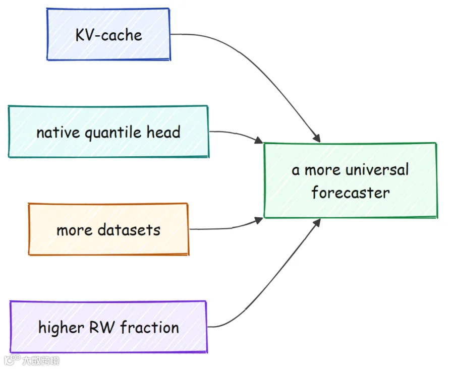
这些都不是深层架构问题。它们是接下来四项工作，每项都有清晰路径。

我们构建的模型是可靠的、校准的、有竞争力的，而且还留下了明显的成长空间。

构建过程教会我的事

同一个教训在每个阶梯上不断出现。17M 阶段，synthetic data 证明了 pipeline，但无法在真实 series 上取胜。

70M 阶段，错误的真实数据输给 naive baseline，正确的数据又 overfit，只有 diversity 和精心设计的 objective 才把它拉回来。起作用的几乎从来不是原始 size，而是 data composition 和 careful measurement；直到 data 和 fixes 到位后，额外 scale 才终于在 200M 上发挥作用。

这就是从零构建这类模型的样子。你不会靠一开始就追求更多参数取胜。

你赢在把数据做对，赢在不自欺地测量，赢在修复那些安静藏在模型最弱位置的 bug；然后，当这一切都成立时，再 scale up，看它落地。我们从一个空文件和一个无法击败的 naive baseline 开始。

最终得到一个从零构建的2 亿参数模型，它能预测从未见过的序列，并带有校准的不确定性。