
哈喽,大家好~
今儿和大家聊聊:决策树回归,又叫回归树、CART 回归~
简单理解,想象在做房价预测,但你不想套一条直线(线性回归)去逼近所有样本。你更希望把数据根据某些“阈值判断”一步一步切分开来:先看“房子是不是在市中心?”,再看“面积是否大于 100 平米?”,再看“是否靠近地铁?”……每一步都是一个“是/否”的问题,最终每个叶子节点会给出一个“平均房价”的预测值。
这样整个模型就是一棵树:从根节点一路往下分裂,直至满足停止条件,叶子节点负责输出预测。
优点是模型直观、能处理非线性、对特征缩放不敏感,解释性强(你可以看到每次为什么这么分)。
缺点也很明显,容易过拟合、对噪声敏感、边界往往是轴平行(即每次只按一个特征阈值分裂),若深度很大,拟合会过细导致泛化差~
数学核心
回归树的目标是在每个节点选择一个特征与阈值,使得分裂后左右两边的“目标值集中程度”更好。回归中常用的衡量“集中程度”的是均方误差(MSE)或方差。设当前节点包含样本集合 ,其目标值为 ,节点的方差定义为:
如果按某特征和阈值将 分成左右两子集 与 ,则这次分裂带来的误差下降量(impurity decrease)为:
训练时我们就是枚举(或近似搜索)所有可能的特征与阈值,寻找能够最大化 的那一对(即最大方差减少)。
叶子的输出通常用叶内样本目标的平均值:
停止条件(常见):
-
达到最大深度:depth >= max_depth -
节点样本数不足:|S| < min_samples_split -
分裂不会带来足够的 impurity decrease(比如小于 min_impurity_decrease) -
或者叶子节点样本小于 min_samples_leaf
超参数就控制着模型的复杂度与泛化能力。
常见超参数与优缺点
-
max_depth(树深度):越深越容易过拟合;浅树容易欠拟合。 -
min_samples_split:一个节点至少需要多少样本才会尝试分裂。 -
min_samples_leaf:叶子至少要有多少样本,能平滑噪声。 -
max_features:每次分裂考虑的特征数量(随机森林常用)。 -
min_impurity_decrease:只有当降幅超过该阈值才分裂(可用于预剪枝)。
优点:
-
易解释:可视化树结构即可看到决策逻辑。 -
能捕捉非线性关系和特征交互。 -
对特征尺度不敏感。
缺点:
-
单颗树通常方差大、泛化能力不如 ensemble(如随机森林、GBDT)。 -
分裂边界是轴平行的(每次只按一个特征阈值分割),对某些复杂边界会产生较多分段近似。
实战案例
说这里我们用 PyTorch 作为数值计算后端(张量操作),并实现一个简化版的回归树(CART 回归)。
我们的数据是二维,方便可视化,目标函数带有非线性与特征交互~
下面给出完整代码与步骤说明(可以复制到 Python 环境运行,需安装 torch、matplotlib、numpy)。
数据生成:两个输入特征 x1, x2,目标函数由非线性项与交互项组成,并加噪声。
我们同时保留一个“真实函数(无噪)”用于比较。
import torch
import numpy as np
import matplotlib.pyplot as plt
from matplotlib import cm
import random

# 为了可重复
seed = 42
random.seed(seed)
np.random.seed(seed)
torch.manual_seed(seed)


def make_data(n=600):
    # X1, X2 分布在 [-3, 3]
    X1 = np.random.uniform(-3, 3, size=n)
    X2 = np.random.uniform(-3, 3, size=n)
    # 真实函数(无噪)
    y_true = np.sin(X1) * X2 + 0.5 * (X1 ** 2) - 0.3 * X2
    # 观测加入噪声
    noise = np.random.normal(0, 1.2, size=n)
    y = y_true + noise
    X = np.vstack([X1, X2]).T
    return X.astype(np.float32), y.astype(np.float32), y_true.astype(np.float32)

X, y, y_true = make_data(600)
X_t = torch.from_numpy(X)  # 用于训练的 torch tensor
y_t = torch.from_numpy(y).unsqueeze(1)
-
目标函数包含 sin、平方、交互项,具有明显的非线性和特征交互,适合展示树的分割效果。 -
我们保留 y_true(无噪)用于对比模型拟合的真实趋势。
实现回归树结构:
class TreeNode:
    def __init__(self, value=None, feature_idx=None, threshold=None, left=None, right=None, is_leaf=False):
        self.value = value          # 叶子预测值
        self.feature_idx = feature_idx
        self.threshold = threshold
        self.left = left
        self.right = right
        self.is_leaf = is_leaf

class DecisionTreeRegressorTorch:
    def __init__(self, max_depth=6, min_samples_split=10, min_samples_leaf=5, min_impurity_decrease=1e-7):
        self.max_depth = max_depth
        self.min_samples_split = min_samples_split
        self.min_samples_leaf = min_samples_leaf
        self.min_impurity_decrease = min_impurity_decrease
        self.root = None
        self.feature_importances_ = None

    def _mse(self, y):
        if y.shape[0] == 0:
            return torch.tensor(0.0)
        mean = torch.mean(y)
        return torch.mean((y - mean) ** 2)

    def _best_split(self, X, y):
        # X: (n, d), y: (n,1)
        n, d = X.shape
        if n < 2:
            return None, None, None, None, None
        best_impurity = self._mse(y)
        best = {'feat': None, 'thr': None, 'left_idx': None, 'right_idx': None, 'impurity_decrease': 0.0}
        for feat in range(d):
            vals = X[:, feat]
            # 选择候选阈值为相邻取值的中点(减少重复计算)
            sorted_idx = torch.argsort(vals)
            vals_s = vals[sorted_idx]
            y_s = y[sorted_idx]
            # candidate thresholds: midpoints where value changes
            diffs = vals_s[1:] - vals_s[:-1]
            valid_positions = torch.nonzero(diffs != 0).squeeze()
            if valid_positions.numel() == 0:
                continue
            thresholds = (vals_s[valid_positions] + vals_s[valid_positions+1]) / 2.0
            # Evaluate each threshold
            for thr in thresholds:
                left_mask = vals <= thr
                right_mask = ~left_mask
                left_count = left_mask.sum().item()
                right_count = right_mask.sum().item()
                if left_count < self.min_samples_leaf or right_count < self.min_samples_leaf:
                    continue
                y_left = y[left_mask]
                y_right = y[right_mask]
                imp_left = self._mse(y_left)
                imp_right = self._mse(y_right)
                weighted_imp = (left_count / n) * imp_left + (right_count / n) * imp_right
                impurity_decrease = best_impurity - weighted_imp
                if impurity_decrease > best['impurity_decrease']:
                    best = {'feat': feat, 'thr': thr.item(),
                            'left_idx': left_mask, 'right_idx': right_mask,
                            'impurity_decrease': impurity_decrease}
        if best['feat'] is None:
            return None, None, None, None, None
        return best['feat'], best['thr'], best['left_idx'], best['right_idx'], best['impurity_decrease']

    def _build(self, X, y, depth=0):
        n = X.shape[0]
        val = torch.mean(y).item()
        # 停止条件
        if depth >= self.max_depth or n < self.min_samples_split or self._mse(y) == 0:
            return TreeNode(value=val, is_leaf=True)
        feat, thr, left_mask, right_mask, imp_dec = self._best_split(X, y)
        if feat is None or imp_dec < self.min_impurity_decrease:
            return TreeNode(value=val, is_leaf=True)
        # 记录特征重要性(累加 impurity decrease)
        if self.feature_importances_ is None:
            self.feature_importances_ = np.zeros(X.shape[1], dtype=np.float64)
        self.feature_importances_[feat] += imp_dec
        left_node = self._build(X[left_mask], y[left_mask], depth+1)
        right_node = self._build(X[right_mask], y[right_mask], depth+1)
        return TreeNode(value=val, feature_idx=feat, threshold=thr, left=left_node, right=right_node, is_leaf=False)

    def fit(self, X_np, y_np):
        X = torch.from_numpy(X_np) if isinstance(X_np, np.ndarray) else X_np
        y = torch.from_numpy(y_np).unsqueeze(1) if isinstance(y_np, np.ndarray) else y_np
        self.feature_importances_ = np.zeros(X.shape[1], dtype=np.float64)
        self.root = self._build(X, y, depth=0)
        # normalize importances
        s = self.feature_importances_.sum()
        if s > 0:
            self.feature_importances_ = self.feature_importances_ / s
        return self

    def _predict_one(self, x, node):
        if node.is_leaf:
            return node.value
        if x[node.feature_idx] <= node.threshold:
            return self._predict_one(x, node.left)
        else:
            return self._predict_one(x, node.right)

    def predict(self, X_np):
        X = X_np if isinstance(X_np, np.ndarray) else X_np.numpy()
        preds = np.array([self._predict_one(x, self.root) for x in X])
        return preds
代码中,使用均方误差(MSE)作为分裂的 impurity 衡量。
对每个特征尝试候选阈值(取相邻不同数值的中点),计算左右子集的 MSE 加权和,选择能够最大化 impurity 减少(方差下降)的分裂。
递归构建树直到满足停止条件。
记录每次分裂带来的 impurity decrease,用于计算特征重要性(最后归一化)。
训练模型并查看特征重要性:
# 训练
model = DecisionTreeRegressorTorch(max_depth=6, min_samples_split=10, min_samples_leaf=5)
model.fit(X, y)
print("feature importances:", model.feature_importances_)
可视化
-
原始的散点图(x1, x2)按 y 值着色,反映观测数据分布。 -
真实函数表面(无噪),显示我们想逼近的真实趋势。 -
模型预测表面(在网格上的预测)并叠加训练点,显示树的分段近似与边界。 -
残差热图(pred - y_true),看模型在哪些区域高估/低估。 -
不同树深度比较:depth=1,3,6,12 的预测面并排展示,看欠拟合到过拟合的演化。
画图前准备网格与预测函数:
# 建网格
xx = np.linspace(-3.2, 3.2, 200)
yy = np.linspace(-3.2, 3.2, 200)
XX, YY = np.meshgrid(xx, yy)
grid = np.vstack([XX.ravel(), YY.ravel()]).T.astype(np.float32)

# 真实函数值(无噪声)
def true_fun(x):
    x1 = x[:, 0]
    x2 = x[:, 1]
    return (np.sin(x1) * x2 + 0.5 * (x1 ** 2) - 0.3 * x2).astype(np.float32)

Z_true = true_fun(grid).reshape(XX.shape)
图 1:原始散点(观测 y)
plt.figure(figsize=(8,6))
plt.scatter(X[:,0], X[:,1], c=y, cmap='plasma', s=25, edgecolor='k')
plt.colorbar(label='observed y (with noise)')
plt.title('Scatter of training samples (colored by observed y) - bright colors')
plt.xlabel('x1'); plt.ylabel('x2')
plt.tight_layout()
plt.show()
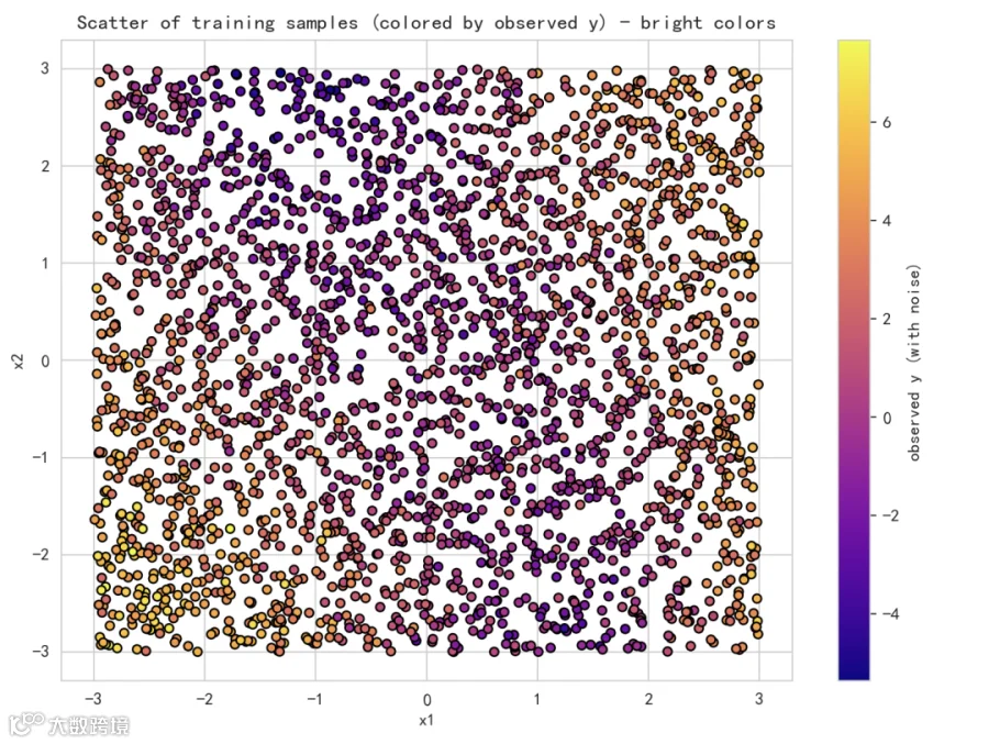
-
每个点的位置由 x1 与 x2 决定,颜色代表观测的目标值 y(含噪)。 -
从颜色可以看出目标值随 x1、x2 的非线性变化趋势和区域性差异。 -
这是模型需要学习的数据分布基础。
图 2:真实函数表面(无噪)
plt.figure(figsize=(8,6))
plt.contourf(XX, YY, Z_true, levels=60, cmap='viridis')
plt.colorbar(label='true y (no noise)')
plt.title('True underlying function (no noise)')
plt.xlabel('x1'); plt.ylabel('x2')
plt.tight_layout()
plt.show()
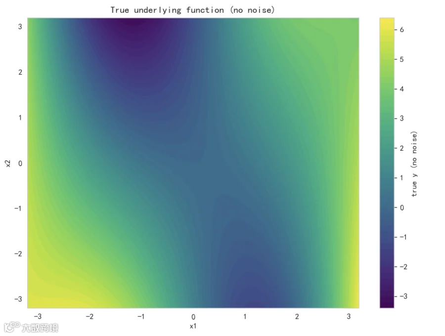
-
这张图展示了我们生成数据时的真实数学关系(无噪)。 -
与图 1 比较可看出噪声导致观测颜色更“杂”,但总体趋势应与此图一致。模型理想上能逼近该表面。
图 3:模型预测表面(单模型,当前 max_depth=6)
Z_pred = model.predict(grid).reshape(XX.shape)

plt.figure(figsize=(8,6))
plt.contourf(XX, YY, Z_pred, levels=60, cmap='plasma')
plt.colorbar(label='predicted y (tree, depth=6)')
# overlay training points
plt.scatter(X[:,0], X[:,1], c=y, cmap='coolwarm', s=18, edgecolor='k')
plt.title('Decision Tree Regression prediction surface (depth=6) with training points')
plt.xlabel('x1'); plt.ylabel('x2')
plt.tight_layout()
plt.show()
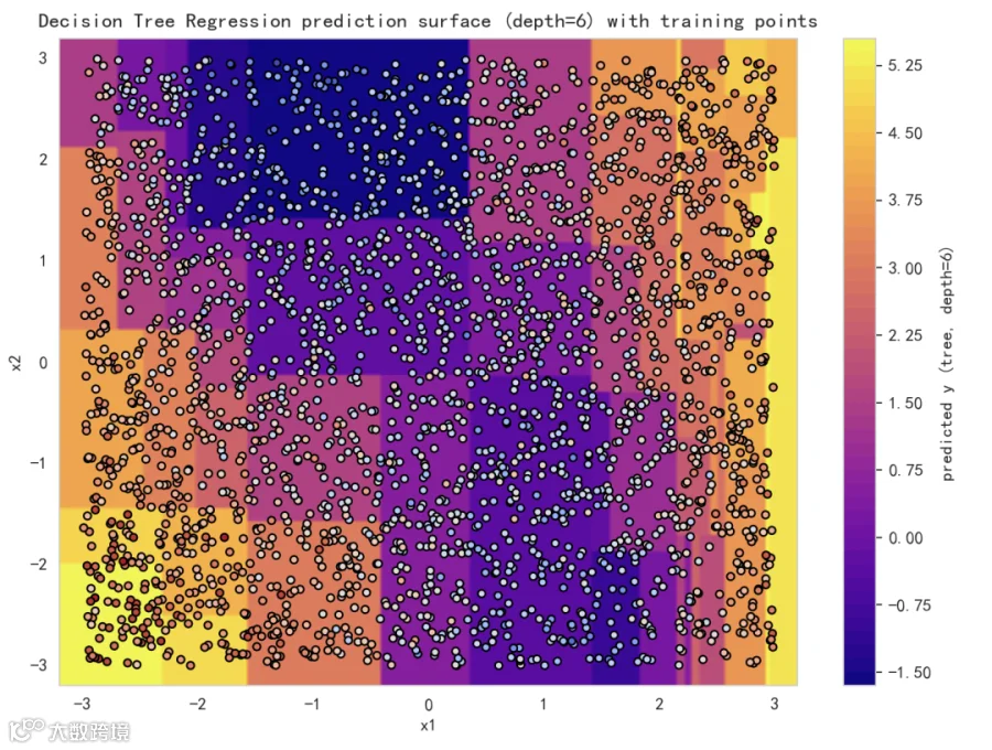
-
这张图显示了树在二维空间上的预测面。注意:树会产生“平整的分块”区域(轴平行边界),这是决策树的典型特征。 -
叠加的训练点能帮助我们看模型是否在噪声样本处过拟合,或在哪些区域拟合欠佳。
图 4:残差(pred - true)热图
Z_resid = Z_pred - Z_true

plt.figure(figsize=(8,6))

plt.contourf(XX, YY, Z_resid, levels=60, cmap='coolwarm', vmin=-np.max(np.abs(Z_resid)), vmax=np.max(np.abs(Z_resid)))
plt.colorbar(label='residual (pred - true)')
plt.title('Residual heatmap (pred - true)')
plt.xlabel('x1'); plt.ylabel('x2')
plt.tight_layout()
plt.show()
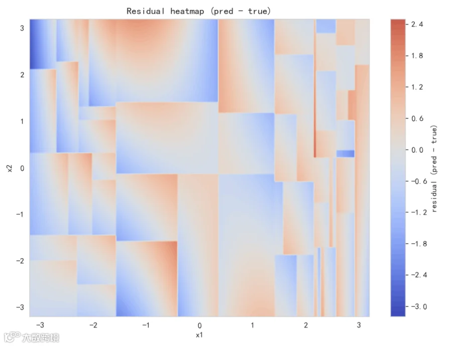
-
残差图显示模型在哪些区域高估或低估。 -
若残差呈结构化(不是纯随机),说明模型未完全捕捉某些趋势;若残差随机、幅度小,说明拟合较好。 -
残差还能提示是否需要更复杂模型或更多数据。
图 5:不同 max_depth 比较(1, 3, 6, 12)
depths = [1, 3, 6, 12]
fig, axs = plt.subplots(1,4, figsize=(20,4))
for ax, d in zip(axs, depths):
m = DecisionTreeRegressorTorch(max_depth=d, min_samples_split=10, min_samples_leaf=5)
m.fit(X, y)
Z = m.predict(grid).reshape(XX.shape)
im = ax.contourf(XX, YY, Z, levels=50, cmap='tab20')
ax.set_title(f'depth={d}')
ax.scatter(X[:,0], X[:,1], c=y, cmap='coolwarm', s=8, edgecolor='k')
ax.set_xticks([]); ax.set_yticks([])
fig.colorbar(im, ax=axs.ravel().tolist(), shrink=0.6)
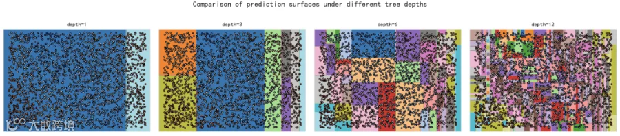
plt.suptitle('Comparison of prediction surfaces under different tree depths', fontsize=16)
plt.tight_layout(rect=[0,0,1,0.95])
plt.show()
-
depth=1:只有一次分裂,模型非常粗糙(欠拟合),预测面大致分为两区。 -
depth=3:可以捕获更多方向的分割,开始逼近一些非线性区域。 -
depth=6:较为细致,可以拟合复杂形状,但可能会在数据稀疏处出现局部波动。 -
depth=12:可能出现过拟合,预测面在很多地方显得“锯齿化”并且紧贴训练点。
除了上面图外,我们还可以输出训练时记录的特征重要性(由 impurity decrease 累积得来):
print("Feature importances (normalized):", model.feature_importances_)
如果某个特征重要性高,说明该特征在分裂时经常被选中并显著降低了叶内方差。
在我们生成的数据里,x1 与 x2 都参与了真实函数,重要性通常都不为零;生成的系数决定了具体贡献大小。
总结
总的来说,单颗回归树易过拟合,实际工程常用集成方法(随机森林、梯度提升树)来降低方差、提高泛化。
另外,决策树对异常值敏感;在数据预处理时注意异常值检测与特征工程。
若特征很多,使用 max_features 可以缓解部分过拟合并引入随机性,对于随机森林尤其重要。