

HelloHello~小伙伴们好,看到这些图,是不是会非常疑惑怎么生成的呢?并且我们平常得到的孟德尔随机化结果都是表格形式,感觉比较普通?所以小记者尝试复现高分文献中的结果图,这样我们可以使用自己的数据,只需要套用代码,就再也不用担心自己的文章里没有精美的图了!
因此,这期给小伙伴们复现两篇文献中孟德尔随机化的结果呈现图,简简单单的几张图,竟然发表了IF15.8+的SCI,让小记者带着大家来学习吧~
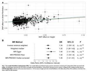
图1
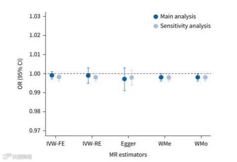
图2
练了十年生信的小记者要凭本事吃饭了,要是您有自己做不了的生信分析,可以联系我~

一、图1复现
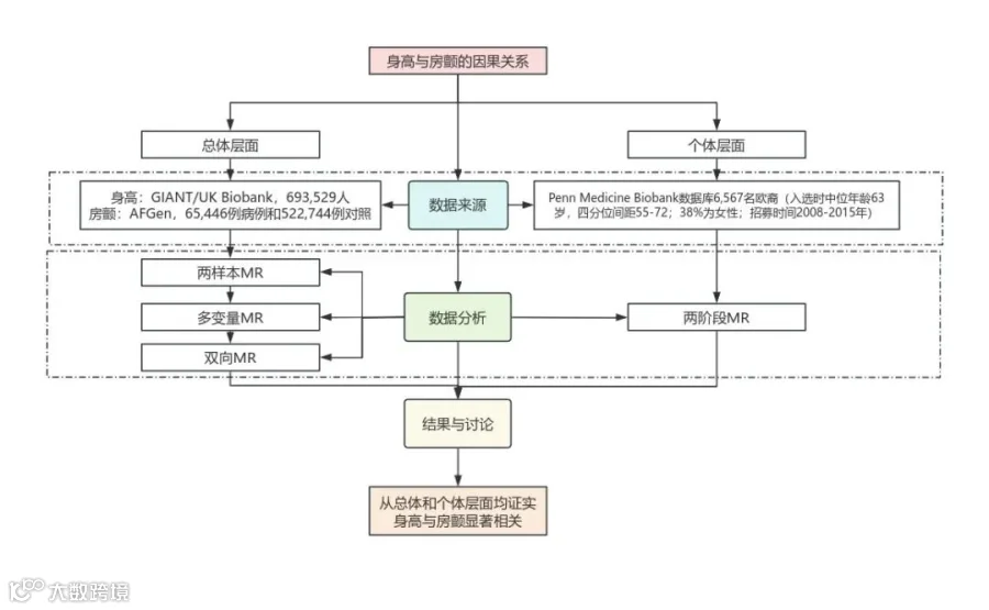
图1来自IF=15.8的《Genetics of height and risk of atrial fibrillation: A Mendelian randomization study》。这篇文献中包含大量的MR结果的散点图和MR分析结果以森林图的形式呈现,更加直观的展示出孟德尔随机化的结果,出图清晰美观。其数据来源及研究思路如下:
总体水平:
身高来源于GIANT/UK Biobank,共693,529人;
房颤来源于AFGen,共65,446例病例和522,744例对照。
个体水平:
Penn Medicine Biobank数据库6,567名欧裔的参与者(入选时中位年龄63岁,四分位间距55-72;38%为女性;招募时间2008-2015年)。
接下来,让我们开始复现吧
#1、散点图和森林图可视化
#导入包library(TwoSampleMR)
接下来从IEU opengwas数据库中得到暴露和结局GWAS数据
#从GWAS上导入暴露数据height与工具变量exposure <- extract_instruments(outcomes = 'ebi-a-GCST90025949',clump = TRUE,r2=0.001,kb=10000,access_token = NULL)#从GWAS上导入暴露数据结局变量房颤与工具变量outcome <- extract_outcome_data(snps = exposure$SNP,outcomes = 'ebi-a-GCST006414',proxies = FALSE,maf_threshold = 0.01,access_token = NULL)
之后效应等位与效应量维持统一,合并为一个数据集
summary <- harmonise_data(exposure_dat = exposure,outcome_dat = outcome)MR分析
result1 <- mr(summary)对结果进行OR值计算
mrOR <- generate_odds_ratios(result1) 绘制散点图
mr_scatter_plot(result1,summary)下面我们开始绘制精美图形啦!
首先导入R包
library(forestploter)library(dplyr)
之后整理数据,并更改变量名为MR_method,OR,P
mrview <- mrOR[,c(5,9,12,13,14)]mrview$se <- (log(as.numeric(mrview$or_lci95)) - log(as.numeric(mrview$or)))/1.96 #se可设置为正方形的大小mrview$` 95% CI` <- ifelse(is.na(mrview$se), "",sprintf("[%.2f - %.2f]",mrview$or_lci95, mrview$or_uci95))mrview$` ` <- paste(rep(" ", 6), collapse = " ")mrview <- rename(mrview,MR_method=method,OR=or,P=pval)
最后绘制图形,小伙伴们根据注释修改参数,即可绘制出自己想要的图形。
p <- forest(data = mrview[,c(1,8,3,7,2)], #导入数据lower = mrOR$or_lci95, # 可信区间下限upper = mrOR$or_uci95, # 可信区间上限#sizes = mrview$se #正方形的大小est = mrOR$or, # 估计值ci_column = 2, # “森林”出现在图的第几列ticks_at = seq(1.0,1.6,0.1), #图例显示的数字xlim = c(0.99,1.61), #x轴的范围xlab = "Odds Ratio(95% Confidence Interval)", #x轴标签xlab_adjust = "center",ref_line = 1)plot(p)
复现结果如下:
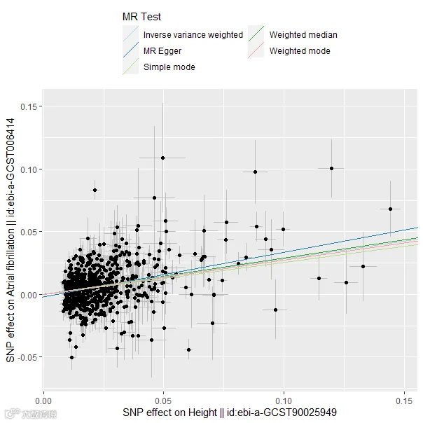
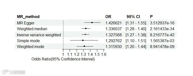
IVW模型发现身高增加与心房颤动显著相关(OR 1.3276;95% CI 1.27-1.38;p=8.2168*e-42),小记者提供的身高和房颤的GWAS数据均来源于IEU opengwas数据库,小伙伴们可以用自己的本地数据进行尝试。看完了第一个,是不是感觉非常简单,让我们一起来下一章图形吧!
温馨小贴士:本次介绍的R包操作占用内存比较大,建议使用服务器,欢迎联系小记者租赁性价比超级高的服务器!!

2、图2复现
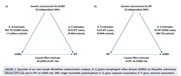
图2来自IF=24.9的《The causal relationship between gastroesophageal reflux disease and idiopathic pulmonary fibrosis: A bidirectional two-sample Mendelian randomization study》。
数据来源
胃食管反流病(Gastro-oesophageal reflux disease,GORD):来自于Ong JS等人关于GORD一项最大的全基因组关联研究(GWAS)的Meta分析,这篇文献IF=24.5,欢迎小伙伴们阅读https://pubmed.ncbi.nlm.nih.gov/34187846/。
特发性肺纤维化(Idiopathic pulmonary fibrosis,IPF):来自于
https://github.com/genomicsITER/PFgenetics。
研究思路
使用目前最大的GORD (病例组78 707例,对照组288 734例)和IPF (病例组4125例,对照组20 464例)全基因组关联荟萃分析的遗传数据,进行双向双样本MR,以估计GORD对IPF风险的因果效应和IPF对GORD风险的因果效应。
MR分析
出图了,出图了,出精美的图了!
首先还是导入所需要的R包
rm(list=ls())library(readr)library(dplyr)library(TwoSampleMR)library(tidyr)library(gwasglue)library(MendelianRandomization)library(simex)library(MRPRESSO)
之后读取胃食管反流病CERD数据——暴露数据
Cerd<-readr::read_tsv("F:/work/2.2/GCST90000514_buildGRCh37.tsv/GastroEsophagealReflux_MTAG_GBME.tsv")cerd1 <- cerd[,c(1,4,5,7,8,9,10)]colnames(cerd1)=c("SNP","effect_allele","other_allele","eaf","beta","se","p")
之后筛选出强相关snp
cerd2 <- subset(cerd1,p<5e-08)cerd2 <- format_data(cerd2,type="exposure",snps = NULL,header = TRUE,snp_col="SNP",beta_col = "beta",se_col = "se",eaf_col = "eaf",effect_allele_col = "effect_allele",other_allele_col = "other_allele",pval_col = "p",log_pval = FALSE)
随后去除连锁不平衡
cerd3 <- clump_data(cerd2,clump_kb = 10000,clump_r2 = 0.001)在之后读取特发性肺纤维化IPF数据——结局数据
ipf <- readr::read_tsv("F:/work/mr出图汇总/GCST90018120_buildGRCh37.tsv/GCST90018120_buildGRCh37.tsv")并且进一步确定强相关的工具变量
ipf1 <- ipf[,c(1,4,5,6,8,9,10)]colnames(ipf1)=c("SNP","effect_allele","other_allele","eaf","beta","se","p")#标准化列名
获取暴露与结局取交集
snps <- intersect(cerd3$SNP,ipf1$SNP)提取交集信息,并提取出暴露和结局数据,exp:暴露数据集;out:结局数据集
exp <- format_data(cerd1,type = "exposure",snps = snps,header = TRUE,snp_col="SNP",beta_col = "beta",se_col = "se",eaf_col = "eaf",effect_allele_col = "effect_allele",other_allele_col = "other_allele",pval_col = "p")out <- format_data(ipf1,type = "outcome",snps = snps,header = TRUE,snp_col="SNP",beta_col = "beta",se_col = "se",eaf_col = "eaf",effect_allele_col = "effect_allele",other_allele_col = "other_allele",pval_col = "p")
之后将暴露与结局合并——等位基因对齐
sum <- harmonise_data(exposure_dat = exp,outcome_dat = out,action = 3)
随后进行5种MR分析,并整合结果
########## IVW fixed effects #########################IVW_FE <- mr_ivw(mr_input(bx = sum$beta.exposure, bxse = sum$se.exposure, by = sum$beta.outcome, byse = sum$se.outcome), model="fixed")ivw1 <- c(IVW_FE@Estimate,IVW_FE@StdError,IVW_FE@CILower,IVW_FE@CIUpper)########## IVW multiplicative random effects #########IVW_RE <- mr_ivw(mr_input(bx = sum$beta.exposure, bxse = sum$se.exposure, by = sum$beta.outcome, byse = sum$se.outcome),model="random")ivw2 <- c(IVW_RE@Estimate,IVW_RE@StdError,IVW_RE@CILower,IVW_RE@CIUpper)########## MR-Egger ##################################Egger <- mr_egger(mr_input(bx = sum$beta.exposure, bxse = sum$se.exposure, by = sum$beta.outcome, byse = sum$se.outcome))egger1 <- c(Egger@Estimate,Egger@StdError.Est,Egger@CILower.Est,Egger@CIUpper.Est)########## Weighted MR median ########################WMe <- mr_median(mr_input(bx = sum$beta.exposure, bxse = sum$se.exposure, by = sum$beta.outcome, byse = sum$se.outcome),weighting = "weighted", iterations = 10000)wme1 <- c(WMe@Estimate,WMe@StdError,WMe@CILower,WMe@CIUpper)########## Mode-based MR #############################WMo <- mr_mbe(mr_input(bx = sum$beta.exposure, bxse = sum$se.exposure, by = sum$beta.outcome, byse = sum$se.outcome), phi=1,iterations=100)wmo1 <- c(WMo@Estimate,WMo@StdError,WMo@CILower,WMo@CIUpper)mr.res <- data.frame(ivw1,ivw2,egger1,wme1,wmo1)mr_heterogeneity(sum) #异质性检验mr_pleiotropy_test(sum) #水平多效性检验
最后就是整理MR分析结果数据以及绘制图形啦!
library(ggplot2)#导入R包mr.res <- t(mr.res) #转置colnames(mr.res) <- c("Estimate","StdError","CILower","CIUpper") #重命名mr.res <- data.frame(mr.res) #数据框形式mr.res$OR <- exp(mr.res$Estimate)mr.res$CL <- exp(mr.res$CILower)mr.res$CU <- exp(mr.res$CIUpper)mr.res$var <- row.names(mr.res) #整理绘图需要的OR及95%CI及变量名
终于到最后一步的绘图了,小伙伴们是不是非常激动~
t <- c("Main analysis")a <- ggplot(mr.res,aes(x=factor(mr.res$var),y=mr.res$OR,fill=t))+geom_point(size=4,colour="blue4")+geom_errorbar(aes(ymax=mr.res$CU,ymin=mr.res$CL),width=0.1,col="blue4")+geom_hline(yintercept = 1,linetype = 2)+theme_set(theme_bw())+theme(panel.grid.major = element_blank(),panel.grid.minor = element_blank())+theme_classic()+ xlab("MR estimators")+theme(axis.title.x = element_text(size=15,vjust = 0.5,hjust = 0.5))+theme(axis.text.x = element_text(size = 10,face = "bold"))+ #x坐标的标签字体设置ylab("OR(95%CI)")+theme(axis.title.y = element_text(size = 15,vjust = 0.5,hjust = 0.5))+theme(axis.text.y = element_text(size = 10,face = "bold"))+ #y坐标的标签字体设置scale_y_continuous(breaks = seq(0.97,1.03,by=0.01),limits = c(0.97,1.03))+labs(colour="Main analysis")+scale_color_manual(values = c("Main analysis"="blue4"))+theme(legend.position = c(1,1),legend.justification = c(1,1))+guides(fill=guide_legend(title=NULL)) #设置图例位置,删除图例标题print(a)
复现结果如下:
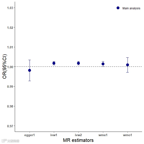
小记者的GORD和IPF数据均来源于GWAS Catalog数据库,图中的缩写全程为IVW-FE: inverse variance weighted fixed effect(ivw1); IVW-RE: inverse variance weighted random effect(ivw2); WMe: weighted median; Egger: MR-Egger; WMo: weighted mode-based。
IVW-FE和IVW-RE结果显示,胃食管反流病与特发性肺纤维化风险显著相关(OR: 1.0017818;95% CI: 1.0008648-1.0027000; p:0.00013895),由图中可以观察到IVW-FE、IVW-RE和WMe的结果均不包含1,因此有统计学意义;MR-Egger和EMo包含1,因此暂不能认为无意义,可能由于样本量等其他因素干扰,影响结果。
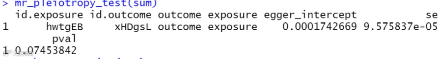
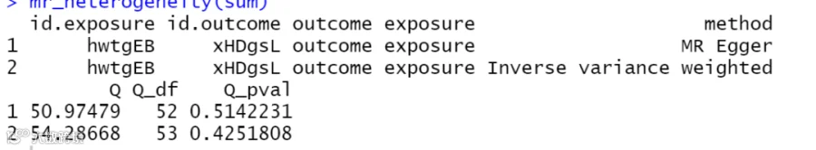
异质性检验和水平多效性检验的p>0.05,因此不存在异质性和水平多效性,因此,没有进一步删除工具变量SNP进行敏感性分析,仅复现部分图形。
不试不知道,一试吓一跳!竟然还有出图如此漂亮的工具,小记者在这里悄悄告诉大家——云生信小程序http://www.biocloudservice.com/home.html!!

小记者话生信
如果您的时间和精力有限或者缺乏相关经验,并且对生信分析和期刊推荐有所需要的话,“生信日报”非常乐意为您提供如下服务:免费思路评估、付费生信分析和方案设计以及付费选刊等,有意向的小伙伴欢迎咨询小记者哦!

生信分析
思路设计
服务器租赁
扫码咨询小记者

1、超高分sci!将近50分你还有不看的理由?德国学者真是把机器学习玩出花了,直接构建一个新生信分析方法,还不快看!
2、国自然出品就是牛!复旦大学施思&虞先濬团队:借公共数据库+RNA-seq+湿实验研究癌症成纤维,IF近9分属实佩服!
3、MDPI期刊再爆丑闻!23本期刊存在“审稿人工厂”问题!