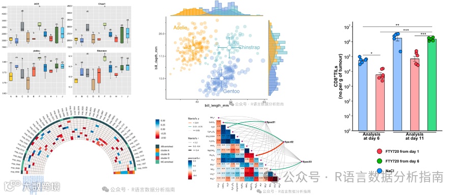


[论文分享] ggplot2绘制炫彩柱状图，点亮你的数据可视化

R语言数据分析指南

2025-04-04

导读：欢迎关注R语言数据分析指南❝本节通过NC上一篇论文的数据来介绍如何绘极坐标柱状图图。

欢迎关注R语言数据分析指南

❝
本节通过NC上一篇论文的数据来介绍如何绘极坐标柱状图图。论文作者有提供对应的代码+数据，小编在其基础上进行了略微的调整，与原文有所出入仅供参考，关于此图的更加详细的介绍请参考论文内容。有需要学习R语言绘图的朋友可关注文末介绍购买小编的R绘图文档。购买前请咨询，零基础不要买。

论文信息

Global floating kelp forests have limited protection despite intensifying marine heatwave threats

Arafeh-Dalmau, N., Villaseñor-Derbez, J.C., Schoeman, D.S. et al. Global floating kelp forests have limited protection despite intensifying marine heatwave threats. Nat Commun 16, 3173 (2025). https://doi.org/10.1038/s41467-025-58054-4

代码下载

https://zenodo.org/records/14796879

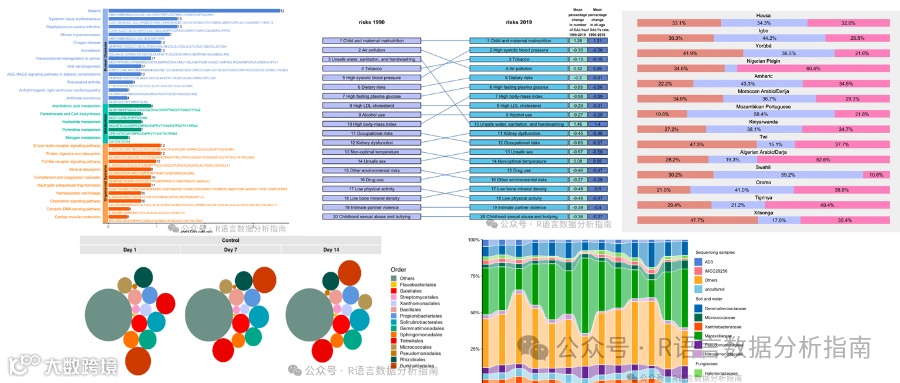
结果图

图形解读

❝
此图为极坐标堆砌条形图，绘制起来难度较小。其主要在于细节的调整如通过geomtextpath来添加文本

代码展示

library(tidyverse)
library(geomtextpath)

labs <- tibble(x = 1,
  y = c(0.1, 0.3) + 0.05,
  label = c("10%", "30%"))

realm_data2 <- realm_data %>% 
  mutate(REALM = str_replace_all(REALM, " ", "\n"))

realm_plot <- ggplot(data = realm_data2)+
  geom_col(aes(x = REALM, y = pct_area, fill = lfp_cat),
           color = "black",linewidth = 0.1) +
  geom_hline(yintercept = 0,linewidth = 0.3)+
  geom_hline(yintercept = 0.1,linetype = "dotted",linewidth = 0.3) +
  geom_hline(yintercept = 0.3,linetype = "dashed",linewidth = 0.3) +
  geom_hline(yintercept = 1,linewidth = 0.3) +
  geom_textpath(data = realm_data2 %>%
                  select(REALM) %>%distinct(),
                mapping = aes(x = REALM,y = 0.75,label = REALM),
                inherit.aes = F,size =3)+
  scale_x_discrete(labels = NULL) +
  scale_y_continuous(limits = c(-0.25, NA),
                     expand = c(0, 0),labels = NULL) +
  scale_fill_manual(values = pal) +
  geom_textpath(data = labs,
            mapping = aes(x = x,y = y,label = label),
            size = 3,inherit.aes = F) +
  coord_polar() +
  theme_void() +
  theme(legend.position = "None") +
  labs(x =NULL,y =NULL,
        fill = "Fishing restrictions")

country_plot <- ggplot(data = country_data) +
  geom_col(aes(x = country,y = pct_area,fill = lfp_cat),
           color = "black",linewidth = 0.1) +
  geom_hline(yintercept = 0,linewidth = 0.3) +
  geom_hline(yintercept = 0.1,linetype = "dotted",
             linewidth = 0.3) +
  geom_hline(yintercept = 0.3,linetype = "dashed",linewidth = 0.3) +
  geom_hline(yintercept = 1,linewidth = 0.3) +
  geom_textpath(data = country_data %>%
              select(country) %>% distinct(),
            mapping = aes(x = country,y = 0.75,
                          label = country),
            inherit.aes = F,size = 3) +
  scale_x_discrete(labels = NULL) +
  scale_y_continuous(limits = c(-0.25, NA),
                     expand = c(0, 0),
                     labels = NULL) +
  scale_fill_manual(values = pal) +
  geom_textpath(data = labs,
            aes(x = x, y = y, label = label),
            size = 3,inherit.aes = F) +
  coord_polar() +
  theme_void() +
  theme(axis.text = element_text(size = 7),
        legend.position = "None") +
  labs(x =NULL,y =NULL,
       fill = "Fishing restrictions")

library(patchwork) # 拼图
(realm_plot|country_plot)+
  plot_annotation(tag_levels = 'A')