
jinzhao:用户增长手册--1. 数据指标体系
jinzhao:用户增长手册--2. 用户分群
jinzhao:用户增长手册--4. 用户流失预测
jinzhao:用户增长手册--3.用户生命周期价值预测
jinzhao: 用户增长手册--5. 预测下一个购买日
jinzhao: 用户增长手册--6. 策略综合收益建模
jinzhao:用户增长手册--7.销量预测
jinzhao: 用户增长手册--8. 预测促销活动的增量收益
用户增长手册--3.用户生命周期价值预测
=================
XGBoost多分类的LTV预测

第3部分:客户生命周期价值 在上一篇文章中,我们对客户进行了细分,找出谁是最好的客户。现在是时候衡量我们应该密切跟踪的最重要的指标之一:客户生命周期价值。我们对客户进行投资(购置成本,离线广告,促销,折扣等),以产生收入并实现盈利。当然,这些行为使某些客户在生命周期价值方面具有超高价值,但总有一些客户降低了盈利能力。我们需要确定这些行为模式,细分客户并采取相应的行动。计算寿命值是容易的部分。首先,我们需要选择一个时间窗口。可能是3、6、12、24个月。通过以下等式,我们可以在特定的时间范围内获得每个客户的生命周期价值:
终生价值:总收入-总费用
为什么要预测:
现在,该等式为我们提供了历史生命价值。如果我们从历史上看到一些客户具有很高的负生命周期价值,那么采取行动可能为时已晚。在这一点上,我们需要通过机器学习来预测未来:
我们将建立一个简单的机器学习模型,以预测客户的终生价值。
2. 终生价值预测
在此示例中,我们还将继续使用我们的在线零售数据集。让我们确定我们的数据探索之路:
为客户生命周期价值计算定义适当的时间范围
确定我们将用来预测未来所需要的数据特征
计算生命价值(LTV)以训练机器学习模型
建立并运行机器学习模型
检查模型是否有用
1. 时间范围
确定时间范围实际上取决于您的行业,业务模型,策略等。对于某些行业来说,一年是很长的时期,而对于另一些行业来说,这是很短的时期。在我们的示例中,我们将进行6个月。每个客户ID的RFM分数(我们在上一篇文章中计算出)是数据集的理想选择。为了后续模型的实现,我们需要拆分数据集。我们将获取3个月的数据,计算RFM并将其用于预测接下来的6个月。因此,我们需要先创建两个数据框,然后将RFM分数附加到它们。
我们已经创建了RFM评分,现在我们的功能集如下所示:
#import libraries
from datetime import datetime, timedelta,date
import pandas as pd
%matplotlib inline
from sklearn.metrics import classification_report,confusion_matrix
import matplotlib.pyplot as plt
import numpy as np
import seaborn as sns
from __future__ import division
from sklearn.cluster import KMeans


import plotly.plotly as py
import plotly.offline as pyoff
import plotly.graph_objs as go

import xgboost as xgb
from sklearn.model_selection import KFold, cross_val_score, train_test_split

import xgboost as xgb

#initate plotly
pyoff.init_notebook_mode()

#read data from csv and redo the data work we done before
tx_data = pd.read_csv('data.csv')
tx_data['InvoiceDate'] = pd.to_datetime(tx_data['InvoiceDate'])
tx_uk = tx_data.query("Country=='United Kingdom'").reset_index(drop=True)

#create 3m and 6m dataframes
tx_3m = tx_uk[(tx_uk.InvoiceDate < date(2011,6,1)) & (tx_uk.InvoiceDate >= date(2011,3,1))].reset_index(drop=True)
tx_6m = tx_uk[(tx_uk.InvoiceDate >= date(2011,6,1)) & (tx_uk.InvoiceDate < date(2011,12,1))].reset_index(drop=True)

#create tx_user for assigning clustering
tx_user = pd.DataFrame(tx_3m['CustomerID'].unique())
tx_user.columns = ['CustomerID']

#order cluster method
def order_cluster(cluster_field_name, target_field_name,df,ascending):
    new_cluster_field_name = 'new_' + cluster_field_name
    df_new = df.groupby(cluster_field_name)[target_field_name].mean().reset_index()
    df_new = df_new.sort_values(by=target_field_name,ascending=ascending).reset_index(drop=True)
    df_new['index'] = df_new.index
    df_final = pd.merge(df,df_new[[cluster_field_name,'index']], on=cluster_field_name)
    df_final = df_final.drop([cluster_field_name],axis=1)
    df_final = df_final.rename(columns={"index":cluster_field_name})
 return df_final


#calculate recency score
tx_max_purchase = tx_3m.groupby('CustomerID').InvoiceDate.max().reset_index()
tx_max_purchase.columns = ['CustomerID','MaxPurchaseDate']
tx_max_purchase['Recency'] = (tx_max_purchase['MaxPurchaseDate'].max() - tx_max_purchase['MaxPurchaseDate']).dt.days
tx_user = pd.merge(tx_user, tx_max_purchase[['CustomerID','Recency']], on='CustomerID')

kmeans = KMeans(n_clusters=4)
kmeans.fit(tx_user[['Recency']])
tx_user['RecencyCluster'] = kmeans.predict(tx_user[['Recency']])

tx_user = order_cluster('RecencyCluster', 'Recency',tx_user,False)

#calcuate frequency score
tx_frequency = tx_3m.groupby('CustomerID').InvoiceDate.count().reset_index()
tx_frequency.columns = ['CustomerID','Frequency']
tx_user = pd.merge(tx_user, tx_frequency, on='CustomerID')

kmeans = KMeans(n_clusters=4)
kmeans.fit(tx_user[['Frequency']])
tx_user['FrequencyCluster'] = kmeans.predict(tx_user[['Frequency']])

tx_user = order_cluster('FrequencyCluster', 'Frequency',tx_user,True)

#calcuate revenue score
tx_3m['Revenue'] = tx_3m['UnitPrice'] * tx_3m['Quantity']
tx_revenue = tx_3m.groupby('CustomerID').Revenue.sum().reset_index()
tx_user = pd.merge(tx_user, tx_revenue, on='CustomerID')

kmeans = KMeans(n_clusters=4)
kmeans.fit(tx_user[['Revenue']])
tx_user['RevenueCluster'] = kmeans.predict(tx_user[['Revenue']])
tx_user = order_cluster('RevenueCluster', 'Revenue',tx_user,True)


#overall scoring
tx_user['OverallScore'] = tx_user['RecencyCluster'] + tx_user['FrequencyCluster'] + tx_user['RevenueCluster']
tx_user['Segment'] = 'Low-Value'
tx_user.loc[tx_user['OverallScore']>2,'Segment'] = 'Mid-Value'
tx_user.loc[tx_user['OverallScore']>4,'Segment'] = 'High-Value'
我们已经创建了RFM评分,现在我们的功能集如下所示:

我将不重复RFM评分的细节,如不清楚,请返回看第二部分。
由于我们的特征已准备就绪,因此,我们将为将用于训练模型的每个客户计算6个月的LTV。
因为数据集中没有指定成本。所以收入直接成为我们的LTV。
#calculate revenue and create a new dataframe for it
tx_6m['Revenue'] = tx_6m['UnitPrice'] * tx_6m['Quantity']
tx_user_6m = tx_6m.groupby('CustomerID')['Revenue'].sum().reset_index()
tx_user_6m.columns = ['CustomerID','m6_Revenue']


#plot LTV histogram
plot_data = [
    go.Histogram(
        x=tx_user_6m.query('m6_Revenue < 10000')['m6_Revenue']
 )
]

plot_layout = go.Layout(
        title='6m Revenue'
 )
fig = go.Figure(data=plot_data, layout=plot_layout)
pyoff.iplot(fig)
此代码段计算LTV并绘制其直方图:

直方图清楚地表明我们的客户的LTV为负。我们也有一些异常值。筛选出异常值对于拥有适当的机器学习模型是有意义的。
好的,下一步。我们将合并3个月和6个月的dataframe,以查看LTV和我们拥有的功能集之间的相关性。
以下代码合并了我们的功能集和LTV数据,并绘制了LTV与RFM总体得分
tx_merge = pd.merge(tx_user, tx_user_6m, on='CustomerID', how='left')
tx_merge = tx_merge.fillna(0)

tx_graph = tx_merge.query("m6_Revenue < 30000")

plot_data = [
    go.Scatter(
        x=tx_graph.query("Segment == 'Low-Value'")['OverallScore'],
        y=tx_graph.query("Segment == 'Low-Value'")['m6_Revenue'],
        mode='markers',
        name='Low',
        marker= dict(size= 7,
            line= dict(width=1),
            color= 'blue',
            opacity= 0.8
 )
 ),
        go.Scatter(
        x=tx_graph.query("Segment == 'Mid-Value'")['OverallScore'],
        y=tx_graph.query("Segment == 'Mid-Value'")['m6_Revenue'],
        mode='markers',
        name='Mid',
        marker= dict(size= 9,
            line= dict(width=1),
            color= 'green',
            opacity= 0.5
 )
 ),
        go.Scatter(
        x=tx_graph.query("Segment == 'High-Value'")['OverallScore'],
        y=tx_graph.query("Segment == 'High-Value'")['m6_Revenue'],
        mode='markers',
        name='High',
        marker= dict(size= 11,
            line= dict(width=1),
            color= 'red',
            opacity= 0.9
 )
 ),
]

plot_layout = go.Layout(
        yaxis= {'title': "6m LTV"},
        xaxis= {'title': "RFM Score"},
        title='LTV'
 )
fig = go.Figure(data=plot_data, layout=plot_layout)
pyoff.iplot(fig)
正相关在这里很明显。高RFM分数意味着高LTV。
在建立机器学习模型之前,我们需要确定这种机器学习问题的类型。LTV本身是一个回归问题。机器学习模型可以预测LTV的$值。但是在这里,我们想要LTV细分市场。因为它使操作更具可行性,并且易于与他人沟通。通过应用K-means聚类,我们可以识别我们现有的LTV组并在其之上构建细分。
考虑到此分析的业务部分,我们需要根据客户的预期LTV区别对待客户。在此示例中,我们将应用集群并分为3个细分(细分的数量实际上取决于您的业务动态和目标):
低LTV
中LTV
高LTV
我们将应用K均值聚类来确定细分并观察其特征:
#remove outliers
tx_merge = tx_merge[tx_merge['m6_Revenue']<tx_merge['m6_Revenue'].quantile(0.99)]


#creating 3 clusters
kmeans = KMeans(n_clusters=3)
kmeans.fit(tx_merge[['m6_Revenue']])
tx_merge['LTVCluster'] = kmeans.predict(tx_merge[['m6_Revenue']])

#order cluster number based on LTV
tx_merge = order_cluster('LTVCluster', 'm6_Revenue',tx_merge,True)

#creatinga new cluster dataframe
tx_cluster = tx_merge.copy()

#see details of the clusters
tx_cluster.groupby('LTVCluster')['m6_Revenue'].describe()
我们已经完成了LTV群集,这是每个群集的特征:

平均8.2k LTV时2是最好的,而396k LTV是0时最差的。在训练机器学习模型之前,还需要采取以下步骤:需要做一些功能工程。
我们应该将分类列转换为数字列。
我们将根据标签LTV群集检查功能的相关性。
我们将功能集和标签(LTV)分为X和y。我们使用X来预测y。
将创建培训和测试数据集。训练集将用于构建机器学习模型,我们将模型应用于测试集以查看其实际性能。
下面的代码为我们完成了所有工作:
#convert categorical columns to numerical
tx_class = pd.get_dummies(tx_cluster)

#calculate and show correlations
corr_matrix = tx_class.corr()
corr_matrix['LTVCluster'].sort_values(ascending=False)

#create X and y, X will be feature set and y is the label - LTV
X = tx_class.drop(['LTVCluster','m6_Revenue'],axis=1)
y = tx_class['LTVCluster']

#split training and test sets
X_train, X_test, y_train, y_test = train_test_split(X, y, test_size=0.05, random_state=56)
让我们从第一行开始。get_dummies()方法将分类列转换为0–1表示法。查看该示例的确切功能:

这是我们在getdummies()之前的数据集。我们有一个分类列,即“细分”。应用getdummies()后会发生什么:

段列已消失,但我们有新的数值表示它。我们将其转换为0和1的3个不同的列,并使其可用于我们的机器学习模型。与相关性相关的行使我们拥有以下数据:

我们发现3个月的收入,频率和RFM分数将对我们的机器学习模型有所帮助。由于我们拥有培训和测试集,因此可以构建模型。
#XGBoost Multiclassification Model
ltv_xgb_model = xgb.XGBClassifier(max_depth=5, learning_rate=0.1,objective= 'multi:softprob',n_jobs=-1).fit(X_train, y_train)

print('Accuracy of XGB classifier on training set: {:.2f}'
 .format(ltv_xgb_model.score(X_train, y_train)))
print('Accuracy of XGB classifier on test set: {:.2f}'
 .format(ltv_xgb_model.score(X_test[X_train.columns], y_test)))

y_pred = ltv_xgb_model.predict(X_test)
print(classification_report(y_test, y_pred))
我们使用了一个称为XGBoost的强大ML库为我们进行分类。自从我们有3个小组(集群)以来,它已经成为一种多分类模型。让我们看一下初步结果:
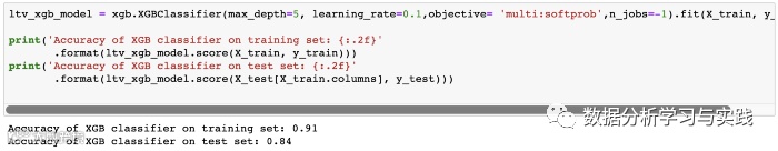
测试仪上的准确度显示为84%。看起来不错。还是需要优化呢?
首先,我们需要检查我们的基准。我们拥有的最大群集是群集0,占总数的76.5%。如果我们盲目地说,每个客户都属于集群0,那么我们的准确性将是76.5%。
84%和76.5%告诉我们,机器学习模型是一种有用的模型,但是肯定需要改进。我们应该找出模型需要改进的地方。我们可以通过查看分类报告来识别这一点:
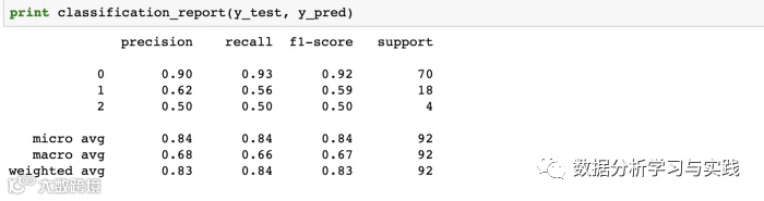
精度和召回率对于0是可接受的。例如,对于集群0(低LTV),如果模型告诉我们该客户属于集群0,则100中的90是正确的(精度)。并且该模型成功识别了93%的实际集群0客户(召回)。我们确实需要改进其他集群的模型。例如,我们几乎没有发现56%的中级LTV客户。可能采取的措施来改善这些问题:
添加更多功能并改善功能工程
尝试XGBoost以外的其他model
将超参数调整应用于当前模型
如果可能,向模型添加更多数据
现在,我们有了一个机器学习模型,该模型可以预测我们客户的未来LTV细分市场。我们可以据此轻松调整我们的行动。例如,我们绝对不希望失去LTV高的客户。因此,在第4部分中,我们将重点关注客户流失预测。
jinzhao:用户增长手册--1. 数据指标体系
jinzhao:用户增长手册--2. 用户分群
jinzhao:用户增长手册--4. 用户流失预测
jinzhao:用户增长手册--3.用户生命周期价值预测
jinzhao: 用户增长手册--5. 预测下一个购买日
jinzhao: 用户增长手册--6. 策略综合收益建模
jinzhao:用户增长手册--7.销量预测
jinzhao: 用户增长手册--8. 预测促销活动的增量收益